Looking for ways to know how you can change to proper case without formula in Excel? Then, this is the right place for you. Here, you will find 6 different step-by-step explained ways of change to proper case without formula in Excel.
How to Change Case to Proper Format without Formula in Excel: 6 Ways
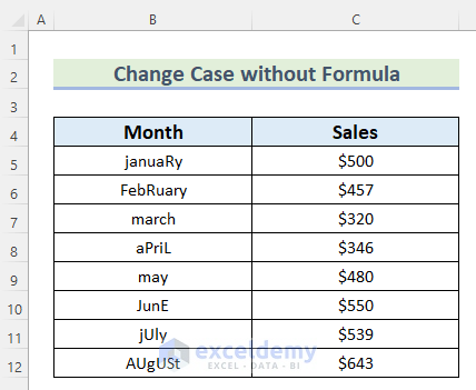
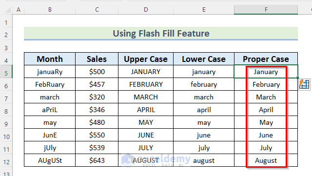
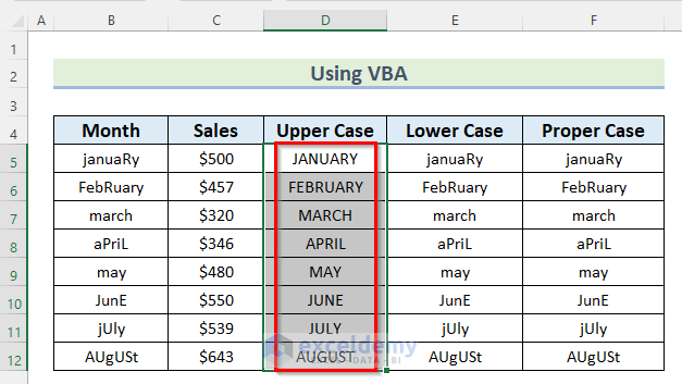
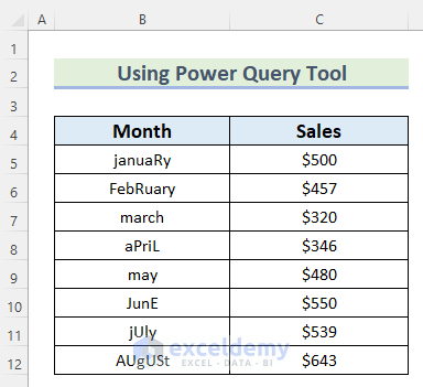
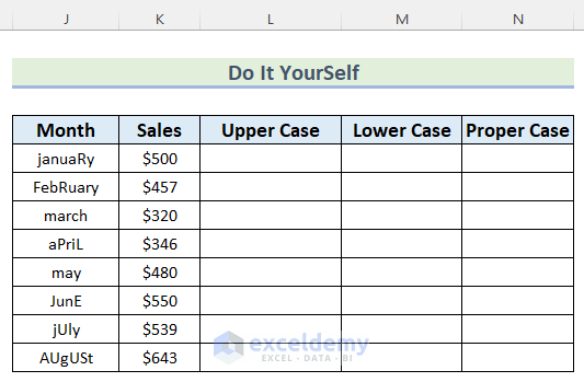
Here, we have a dataset containing the Month and Sales of a store. We will show you how to change to proper case of the months given here without using formulas in Excel.
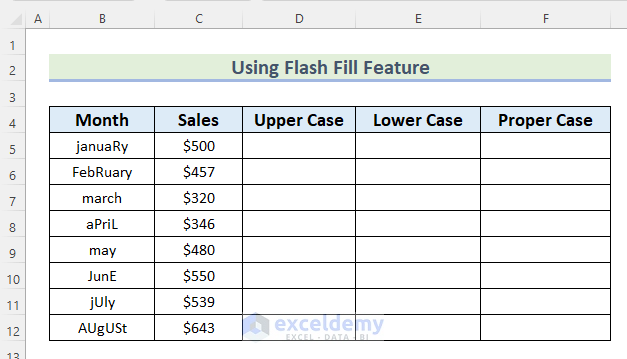
1. Using Flash Fill Feature to Change Case to Proper Format in Excel
In the first method, we will use the Flash Fill Feature to change case to proper format in Excel. Here, in the data, we will change the case of given months to Upper Case, Lower Case, and Proper Case.
Follow the steps given below to do it on your own.
Steps:
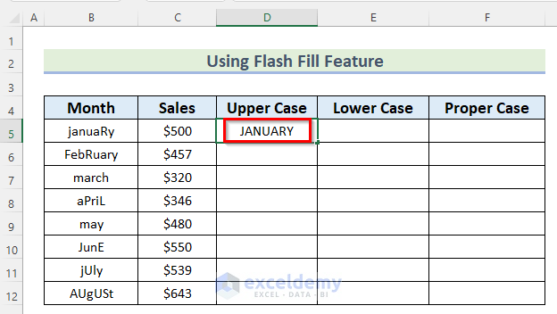
- First, select the Cell D5.
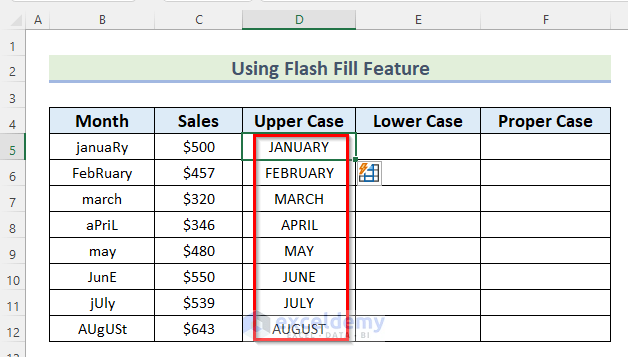
- Then, type “JANUARY” as it is the Upper Case of corresponding Cell B5 it will create a pattern. The Flash Fill feature will follow that pattern to change the case.
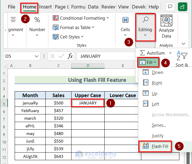
- After that, again select Cell D5.
- Next, go to the Home tab >> click on Editing >> click on Fill >> select Flash Fill.
- Now, you will have all the values of months in Upper Case.
- Next, select Cell E5.
- Then, type “january” as it is the Lower Case of corresponding Cell B5.
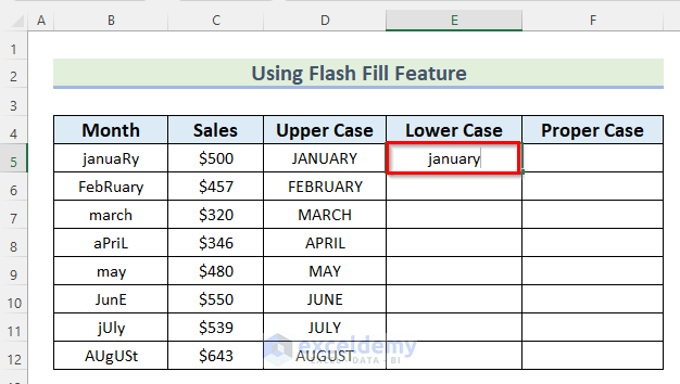
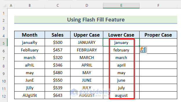
- Similarly, use the Flash Fill feature to get the values in Lower Case as you have done for Upper_Case.
- Then, select Cell F5.
- After that, type “January” as it is the Proper Case of corresponding Cell B5.
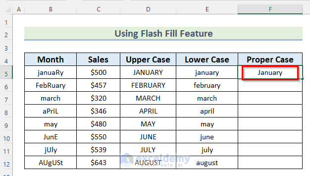
- Again, use the Flash Fill feature to get the values in Proper Case as you have done for Upper_Case.
Read More: How to Change Case in Excel Without a Formula
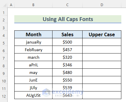
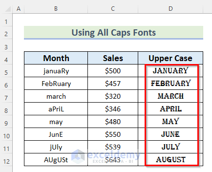
2. Use of All Caps Fonts to Change Case to Proper Format
Now, we will use the All Caps Fonts to change the case of the given months to Upper Case in Excel.
Go through the steps to do it on your own.
Steps:
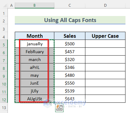
- After that, press CTRL+V to Paste it in Cell range D5:D12.

- Next, select the Cell range D5:D12.
- Then, go to the Home tab >> from Fonts >> click on Theme Fonts.
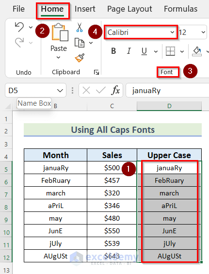
- After that, select any Font that is in All Caps. Here, we will select ALGERIAN as Theme Font.

- Finally, you will get all the values of months in the Upper Case using All Caps Fonts in Excel.
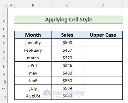
3. Applying Cell Styles Feature to Change Case in Excel
Next, we will use the Cell Styles to change the case to the proper case of the given months to Upper Case in Excel.
Go through the steps to do it on your own dataset.
Steps:
- First, Copy the Cell range B5:B12 and Paste it into Cell range D5:D12 using the same steps done in Method_2.

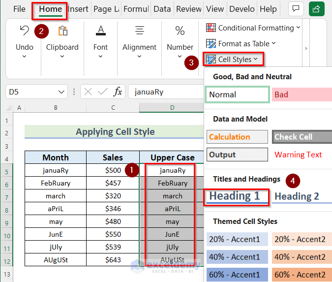
- Then, select the Cell range D5:D12.
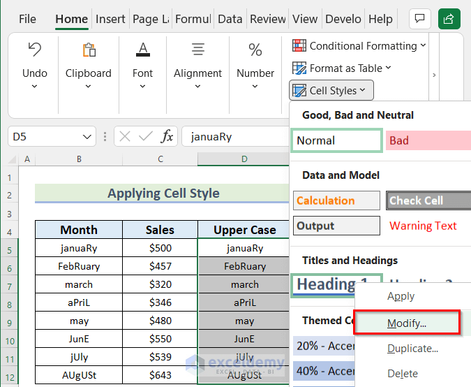
- Afterward, go to the Home tab >> click on Cell Styles >> Right Click on Heading 1.
- Next, click on Modify.
- Now, the Style box will open.
- Then, click on Format.

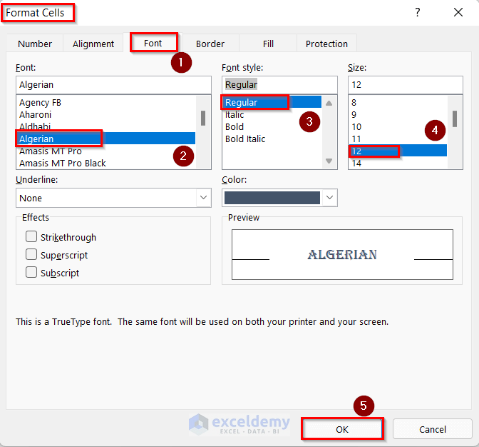
- Now, the Format Cells toolbox will appear.
- After that, go to Fonts >> select Font as Algerian >> select Font style as Regular >> select Size as 12.
- Finally, press OK.
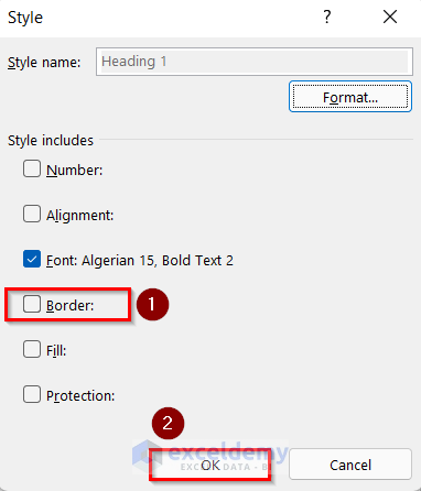
- Then, in the Style box, turn off the Border option.
- After that, press OK.
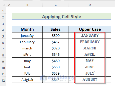
- Finally, you will get all the values of months in Upper Case without using formulas in Excel.
Read More: How to Capitalize All Letters Without Formula in Excel
4. Using Excel VBA to Change Case to Proper Format
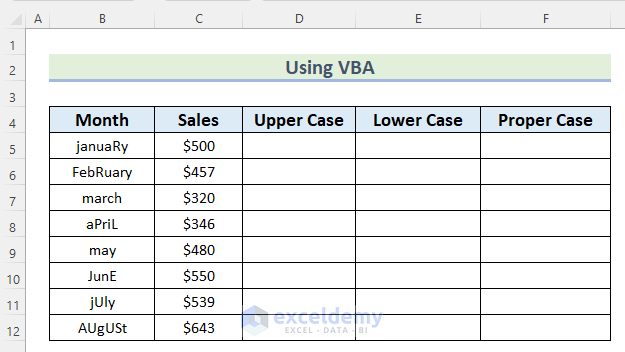
We can also use VBA to change the case of the months into Upper Case, Lower Case, and Proper Case in Excel.
Steps:
- First, Copy Cell range B5:B12 and Paste it into Cell ranges D5:D12, E5:E12, and F5:F12 using the same steps done in Method_2.

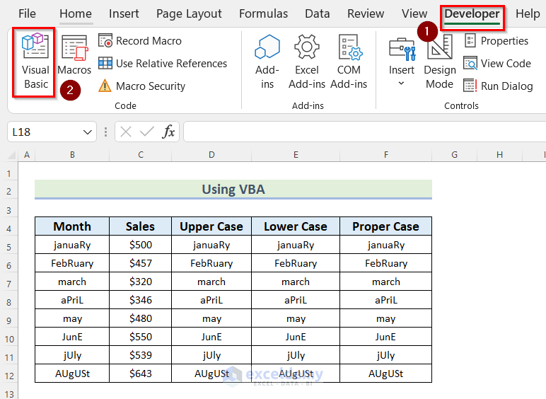
- Then, go to the Developer tab >> click on Visual Basic.
- Now, Microsoft Visual Basic for Application box will open.
- After that, click on Insert >> select Module.

- Then, write the following code in your Module.
Sub upper_case()
For Each unique_cell In Selection
If Not unique_cell.HasFormula Then
unique_cell.Value = UCase(unique_cell.Value)
End If
Next unique_cell
End Sub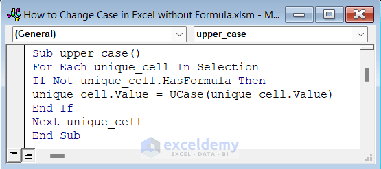
Sub lower_case()
For Each unique_cell In Selection
If Not unique_cell.HasFormula Then
unique_cell.Value = LCase(unique_cell.Value)
End If
Next unique_cell
End Sub
Sub proper_case()
For Each unique_cell In Selection
If Not unique_cell.HasFormula Then
unique_cell.Value = Application.WorksheetFunction.proper(unique_cell.Value)
End If
Next unique_cell
End Sub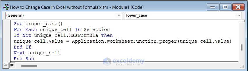
Code Breakdown
- First, we created Sub Procedure as upper_case().
- Then, we used a For loop for each unique_cell in Selection.
- After that, we used the VBA LCase function in the IF statement to change the case into Upper Case.
- Next, we set the same steps for the next unique_cell.
- Similarly, we created Sub Procedure as lower_case() and proper_case().
- Then, we followed the same steps as Upper Case.
- Next, click on the Save button and go back to your worksheet.

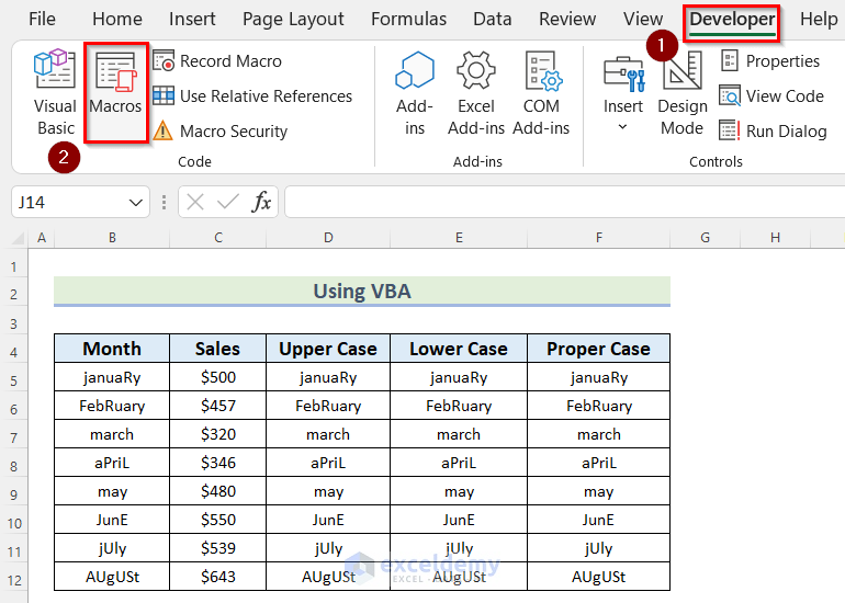
- After that, go to the Developer tab >> click on Macros.
- Now, the Macros box will appear.
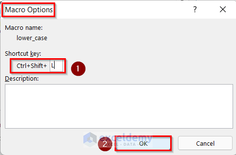
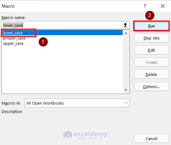
- Then, select lower_case.
- After that, click on Options.

- Then, in the Shortcut key box insert CTRL+SHIFT+L.
- After that, press OK.
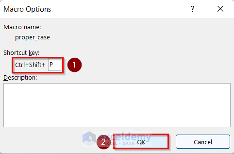
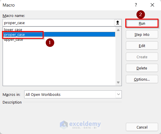
- Next, select proper_case.
- Then, click on Options.

- Now, in the Shortcut key box insert CTRL+SHIFT+P.
- After that, press OK.
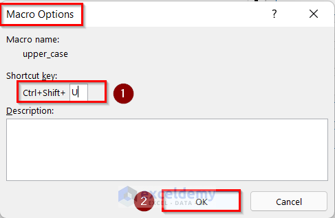
- Finally, select upper_case.
- Next, click on Options.

- Then, in the Shortcut key box insert CTRL+ShHIFT+U.
- After that, press OK.
- Next, select Cell range D5:D12.
- Then, go to the Developer tab >> click on Macros.
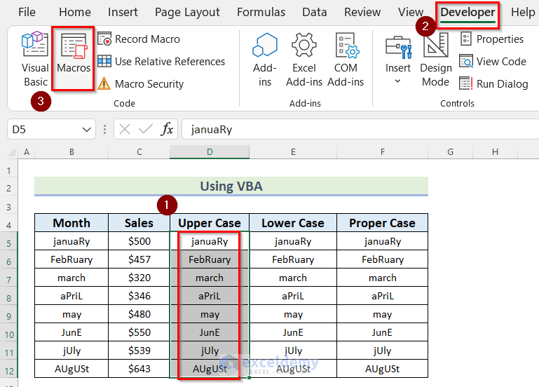
- Now, the Macros box will open.
- Next, select upper_case.
- Then, click on Run.

- After that, you will get all the values of months in Upper Case using VBA in Excel.
You can also do this by directly using a Keyboard Shortcut.
- First, select the Cell range D5:D12.
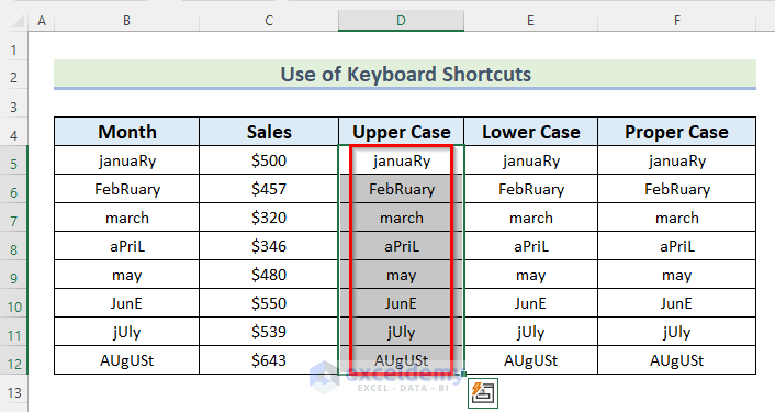
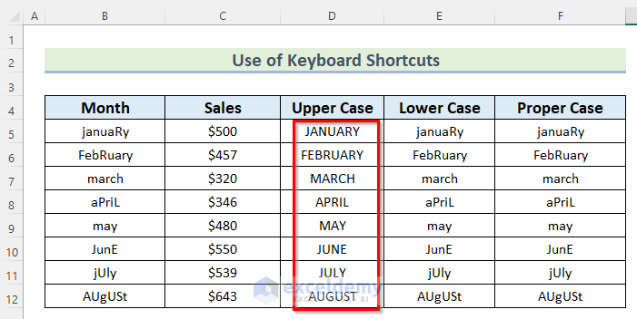
- After that, press the keyboard shortcut CTRL+SHIFT+U.
- Now, you can see all the values of months have changed into Upper Case.
- Next, for Lower Case select Cell range E5:E12.
- Then, go to the Developer tab >> click on Macros.
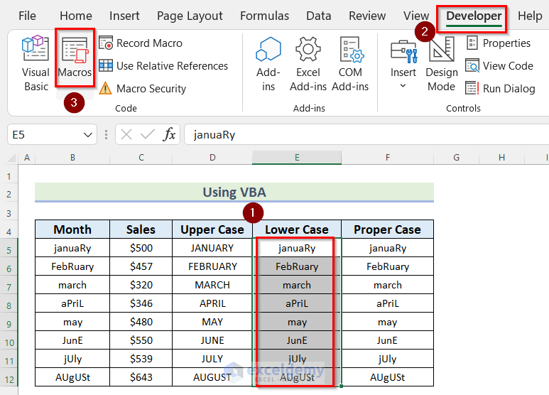
- Again, the Macros box will open.
- Then, select lower_case.
- Next, click on Run.
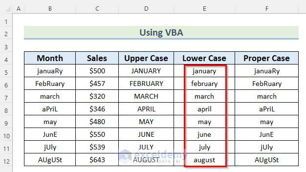
- Then, you will get all the values of months in Lower Case using VBA in Excel.
- Now, we will use Keyboard Shortcut to change the case into Lower Case.
- First, select the Cell range E5:E12.

- Then, press the Keyboard Shortcut CTRL+SHIFT+L.
- Here, you can see all the values of months have changed into Lower Case.

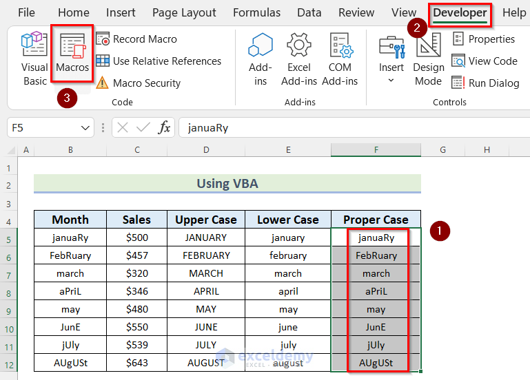
- After that, for Proper Case select Cell range F5:F12.
- Then, go to the Developer tab >> click on Macros.
- Now, the Macros box will open.
- Then, select lower_case.
- Next, click on Run.
- Finally, you will get all the values of months in Proper Case using VBA in Excel.

You can also do it by using a Keyboard shortcut.
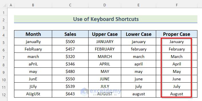
- First, select the Cell range F5:F12.
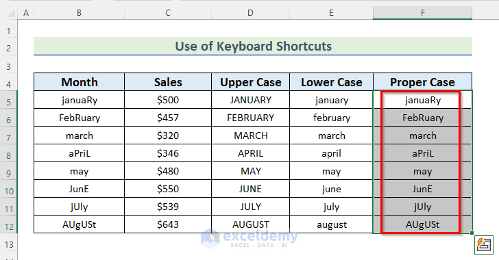
- Now, press the Keyboard Shortcut CTRL+SHIFT+P.
- Finally, you can see all the values of months have changed into Proper Case.
Read More: How to Use VBA in Excel to Capitalize All Letters
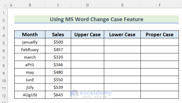
5. Use of Microsoft Word “Change Case” Feature
We can also change cases in Excel with the help of Microsoft Word. Here, we will show you how to use Microsoft Word to change the case of the given months into Upper Case, Lower Case, and Proper Case.
Go through the steps to do it on your own.
Steps:
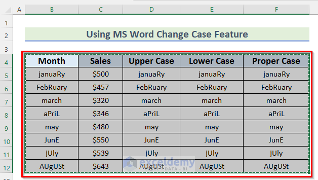
- In the beginning, Copy Cell range B5:B12 and Paste it into Cell ranges D5:D12, E5:E12 and F5:F12 using the same steps done in Method_2.

- Then, select the Cell range B4:F12.
- After That, press CTRL+C to Copy the Cell range.
- Next, open a Microsoft Word file.
- Now, press CTRL+V to Paste the Cell range B4:F12.

- Then, select all the data from the Upper Case column.
- Afterward, go to the Home tab >> click on the Case Change button.
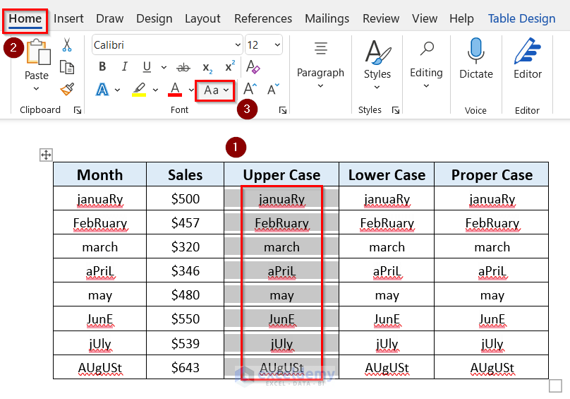
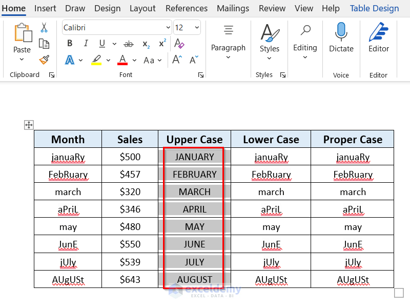
- Next, click on UPPERCASE.

- Now, you will get all the values of months in Upper Case in Microsoft Word.
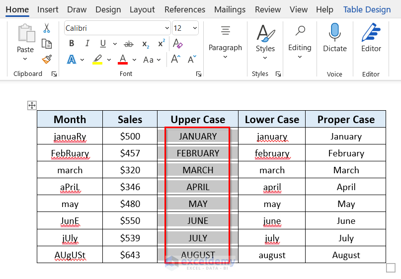
- Then, follow the steps for Lower Case and Proper Case as you have done for Upper Case. Here, For Lower Case and Proper Case select the lowercase and Capitalize Each Word options respectively from the Case Change tool.

- Now, select all the data from the Upper Case column.
- After That, press CTRL+C to Copy all the data.
- Next, go to the Excel file and click on Cell D5.
- Then, press CTRL+V to Paste all the Upper Case data.

- Similarly, Copy and Paste all the data for Lower Case and Proper Case columns from Microsoft Word to Excel.
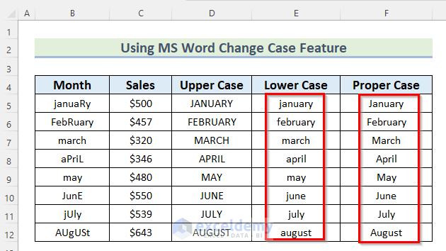
Thus, you will get all the values to months in Upper Case, Lower Case, and Proper Case in Excel with the help of Microsoft Word.
Read More: How to Change Lowercase to Uppercase in Excel Without Formula
6. Using Power Query Tool to Change Case to Proper Format in Excel
In the final method, we will show you how to use the Power Query Tool which will change any case to a proper case without formula in Excel.
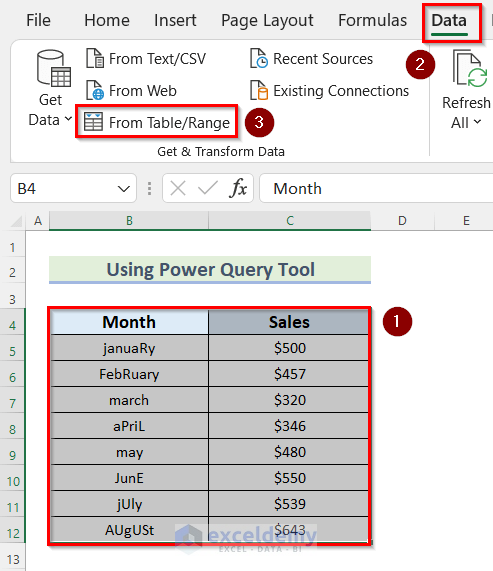
- First, select the Cell range B4:C12.
- Then, go to the Data tab >> click on From Table/Range.
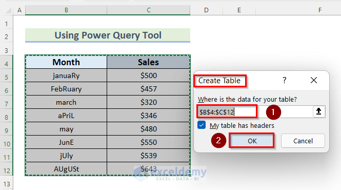
- Now, the Create Table box will open.
- Here, you can see that the Cell range has already been selected.
- My table has headers is selected.
- Then, click on OK.
- Next, the Power Query Editor box will appear.
- Here, you can see the Cell range in Table1 and the Month column is already selected.
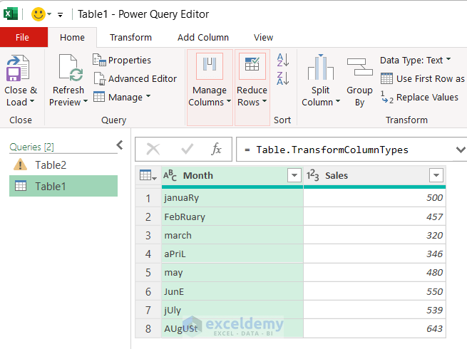
- Then, go to the Add Column tab >> click on Format >> select UPPERCASE.
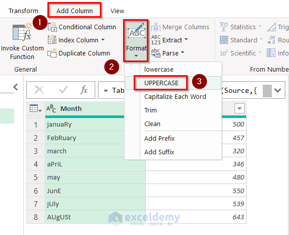
- Then, you will find that a new column containing the values of months in UPPERCASE is created.

- Similarly, select the Month column.
- Next, go to the Add Column tab >> click on Format >> select lowercase.
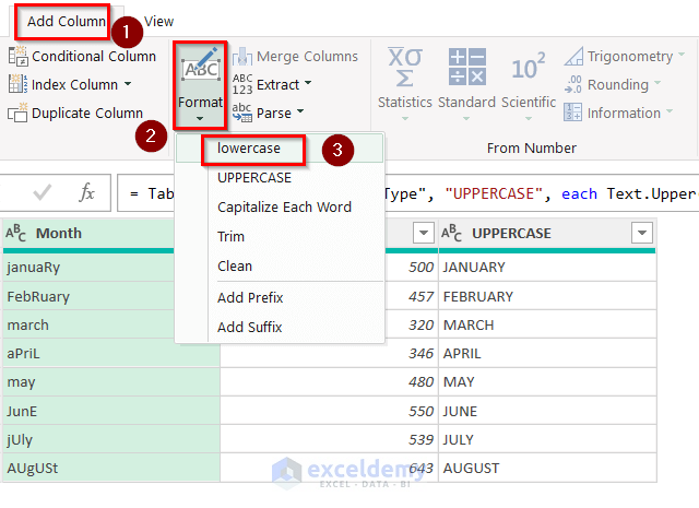
- Now, you will get a new column containing the data of lowercase of the month column.

- Next, select the Month column again.
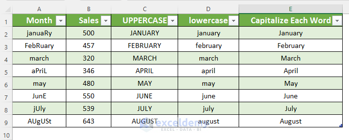
- Then, go to the Add Column tab >> click on Format >> select Capitalize Each Word.

- After that, a new column containing the data of months in Proper Case will be added to the table.

- Next, go to the File tab >> click on Close & Load
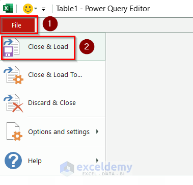
- Finally, we will get the values of months in Upper Case, Lower Case, and Proper Case using the Power Query Tool.
Practice Section
In this section, we are giving you the dataset to practice on your own and learn to use these methods.
Download Practice Workbook
Conclusion
So, in this article, you will find 4 ways that will change to proper case without formula in Excel. Use any of these ways to accomplish the result in this regard. Hope you find this article helpful and informative. Feel free to comment if something seems difficult to understand. Let us know any other approaches which we might have missed here. Thank you!
Related Articles
- How to Change to Title Case in Excel
- Automatic Uppercase in Excel VBA
- How to Stop Auto Capitalization in Excel
<< Go Back to Change Case | Text Formatting | Learn Excel
Get FREE Advanced Excel Exercises with Solutions!
