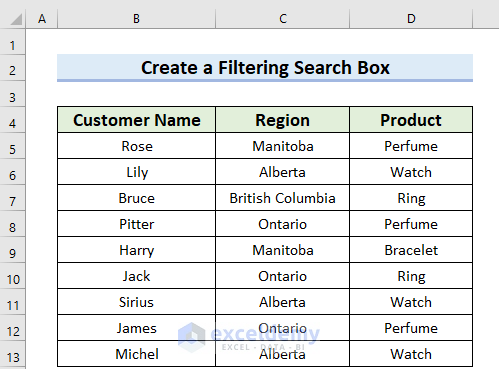
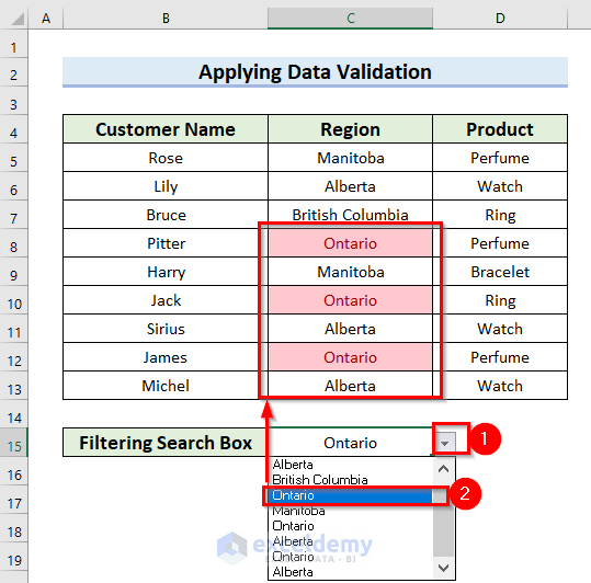
In the below dataset, we have 3 columns: Customer Name, Region and Product.
Method 1 – Using Data Validation
Steps:
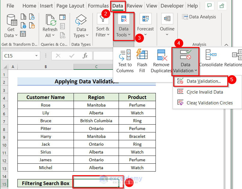
- Select a cell that you want to use as a filtering search box. Here, I have selected cell C15.
- From the Data tab >> go to the Data Tools feature >> choose the Data Validation command >> select Data Validation.
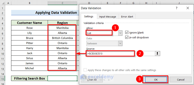
A dialog box named Data Validation will appear.
- Choose the List option from the drop-down arrow in the Allow section.
- In the Source box, select the data range depending on which Filtering will work. Here, I have selected the data range of the Region column.
- Press OK.
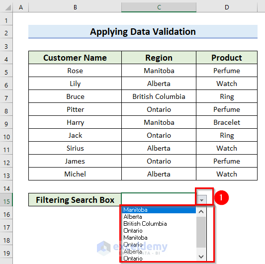
- You will see the filtering search box by clicking on the drop-down arrow of cell C15.
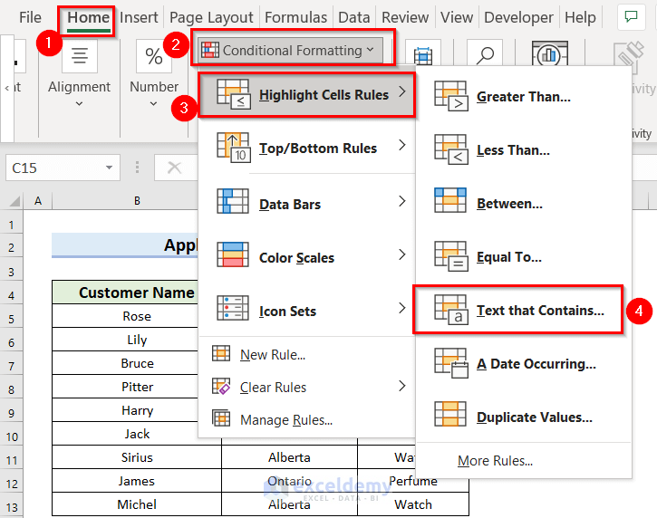
- From the Home tab >> go to the Conditional Formatting command >> choose the Highlight Cells Rules feature >> select Text that Contains...
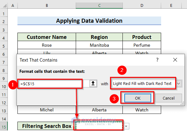
A dialog box named Text That Contains will appear.
- select cell C15 in the Format cells that contain the text: box. Select the cell where you have applied the Data Validation feature, not the cell value.
- Choose the highlight color.
- Press OK.
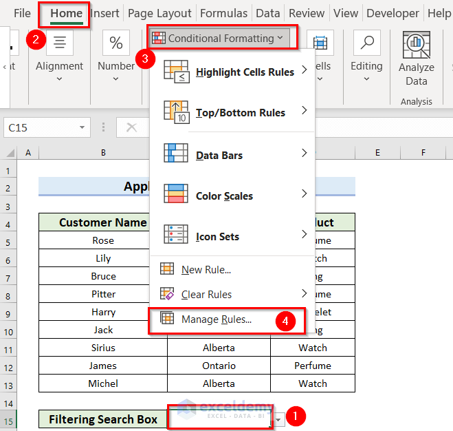
- Select cell C15.
- From the Home tab >> go to the Conditional Formatting command >>Select Manage Rules.
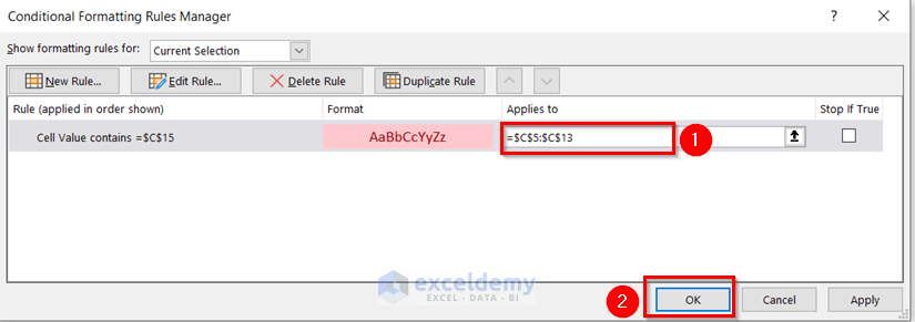
A dialog box, Conditional Formatting Rules Manager, will appear.
- In the Applies to box, select the whole data range. Here, I have selected the range C5:C13.
- Press OK to get the changes.
See the results below. Here, I have created a filtering search box. When I choose the Ontario region, all the cells in the Region column with the same cell values are marked.
Read More: How to Create a Search Box in Excel
Method 2 – Combining Excel Functions
Steps:
- Select the data range.
- From the Insert tab >> choose the Table feature.
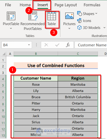
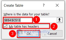
A dialog box named Create Table will appear.
- Select the data range in the Where is the data for your table? box.
- Check the My table has headers option.
- Press OK.
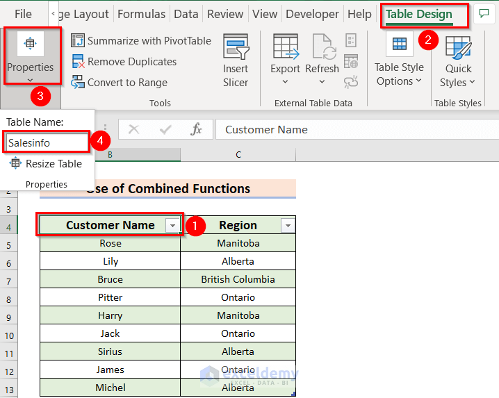
Your table is ready.
- Select any cell of the table.
- From the Table Design tab >> go to the Properties option.
- Enter a table name in the Table Name box. Here, I have written Salesinfo.
- Select a different cell with enough space to keep your whole data.
- Enter the following formula in the cell:
=FILTER(Salesinfo,LEFT(Salesinfo[Region],LEN(F2))=F2,"No Region Found")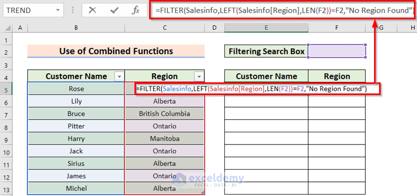
Formula Breakdown
- Cell F2 will be the search box.
- The LEN function returns the total number of characters in cell F2. What you enter in cell F2 will be counted by the LEN function.
- The LEFT function will return the characters from the start of a given text.
- Salesinfo[Region] denotes the Region column from the Salesinfo table.
- The FILTER function filters the data. Here, the array is a table named Salesinfo. It will search for the letters written in cell F2. If there are no such letters, it will return No Region Found.
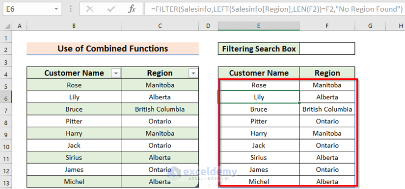
- Press ENTER to get the result.
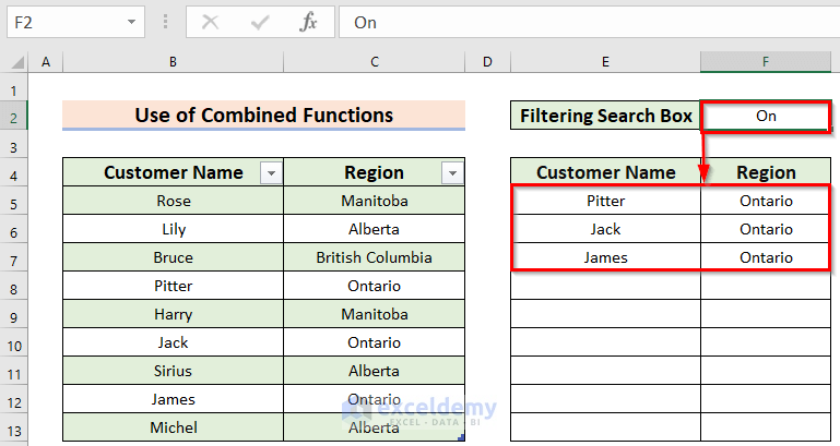
If I write just On, it will give all the Regions whose names start with On letters.
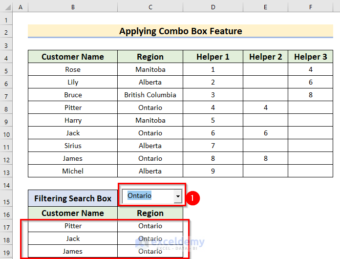
Method 3 – Applying a Combo Box
Steps:
a) Make a List of Unique Regions for Filtering the Search Box
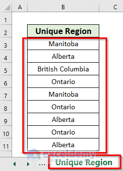
- Copy the data range based on which the filtering search box will work. Here, I have copied the data from the Region column of the previous data set.
- Go to a new worksheet and paste that there. Here, my new worksheet name is Unique Region.
- Select the data range of the Unique Region column.
- From the Data tab >> go to the Data Tools feature >> choose the Remove Duplicates option.
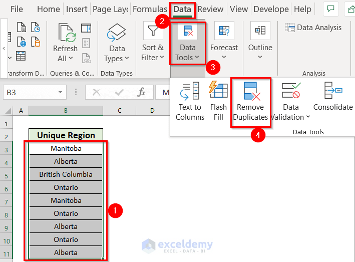
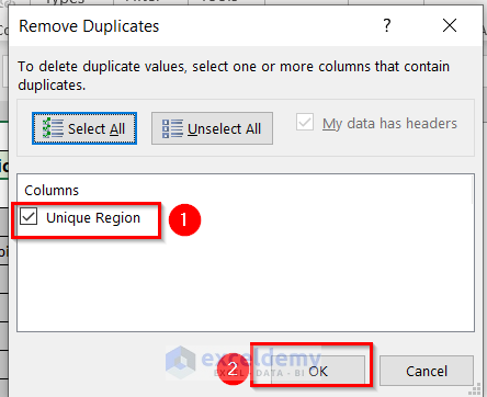
A dialog box named Remove Duplicates will appear.
- Check the Unique Region.
- Press OK.
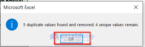
- Press OK on the window named Microsoft Excel.
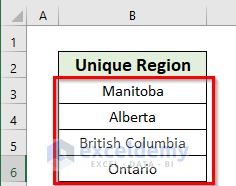
All the Unique Regions are here.
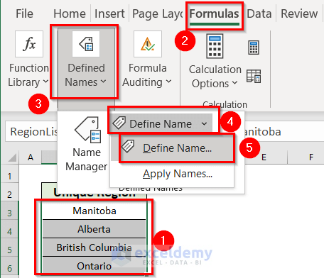
- Select the data of Unique Regions.
- From the Formulas tab >> go to the Defined Names command.
- From the Define Name feature >> choose the Define Name… option.
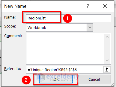
A dialog box named New Name will appear.
- Enter RegionList in the Name box.
- Press OK to keep the changes.
You have defined the name of the Unique Region data as RegionList.
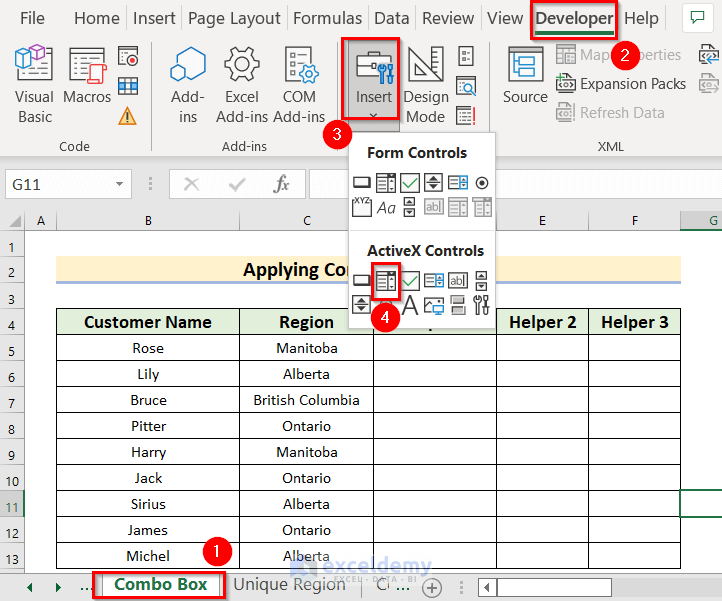
b) Inserting a Combo Box to Create a Dynamic Filtering Search Box
- Go back to the previous worksheet named Combo Box.
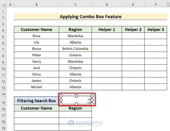
- From the Developer tab >> select the Insert feature >> Insert a Combo Box (ActiveX Controls). Click on the Combo Box (ActiveX Controls) option and then drag the Mouse Pointer at a certain place to insert the Combo Box.
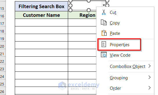
- Right-click on the Combo Box.
- From the Context Menu Bar >> go to the Properties option.
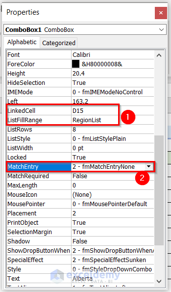
Here, you have to do three things in the Properties window.
- Enter an empty cell like D15 in the LinkedCell box.
- Enter RegionList in the ListFillRange box.
- Select 2- fmMatchEntryNone in the MatchEntry box.
- Close this window.
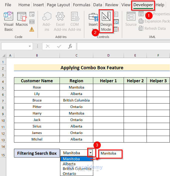
- From the Developer tab >> uncheck the Design Mode feature.
- If you click on the drop-down arrow of the Combo Box, you will see the list of unique regions. If you select any region from that list, you will get that region in cell D15.
- Select a different cell.
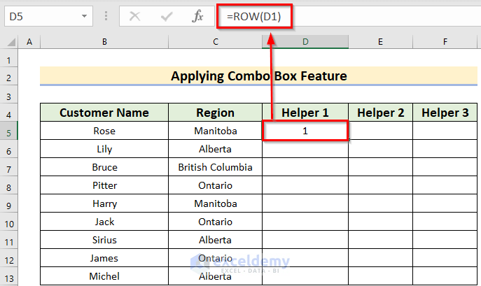
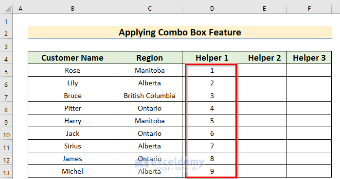
- Enter the following formula in that cell:
=ROW(D1)In this formula, the ROW function will return the row number of a cell.
- Press ENTER to get the result.
- Drag the Fill Handle icon to paste the used formula respectively to the other cells of the column.
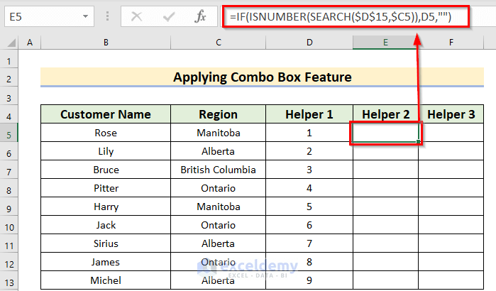
- Select another cell.
- Enter the following formula in that cell:
=IF(ISNUMBER(SEARCH($D$15,$C5)),D5,"")- Press ENTER to get the result.
- Now, select another cell.
- Then write down the following formula in that cell:
=IFERROR(SMALL($E$5:$E$13,ROWS($E$5:E5))," ")- Press ENTER to get the result.
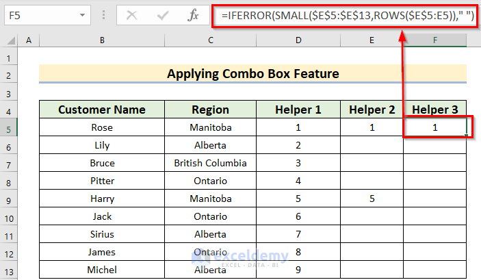
Formula Breakdown
- The ROWS function will count the number of the total rows for a given array.
- ROWS($E$5:E5)—> returns 1.
- The SMALL function will return the k-th smallest value from a given array.
- SMALL($E$5:$E$13,1)—> becomes 1.
- The IFERROR function checks whether the value is an error. If it is, it will give a blank space.
- IFERROR(1,” “)—> turns 1.
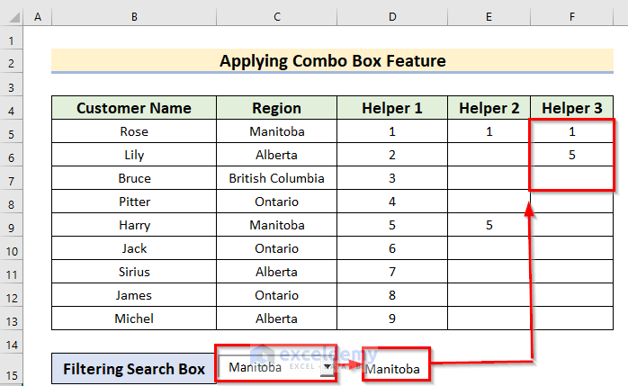
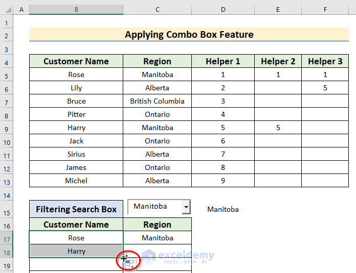
When I selected Manitoba from the Combo Box, the value in cell D15 became Manitoba, too. Then, it sorted the data in the F column based on the D and E columns, where Manitoba was.
- Select another cell.
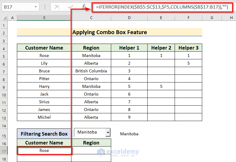
- Enter the following formula in that cell:
=IFERROR(INDEX($B$5:$C$13,$F5,COLUMNS($B$17:B17)),"")- Press ENTER to get the result.
Formula Breakdown
- The COLUMNS function returns the total number of columns of a given array.
- COLUMNS($B$17:B17)—> turns 1.
- The INDEX function returns a searched value. Here, $B$5:$C$13 is the array, and $F5 is the row number.
- INDEX($B$5:$C$13,$F5,1)—> becomes Rose.
- The IFERROR function checks whether the value is an error or not. If it is an error, it will give a blank space.
- Drag the mouse pointer up to cell C17.
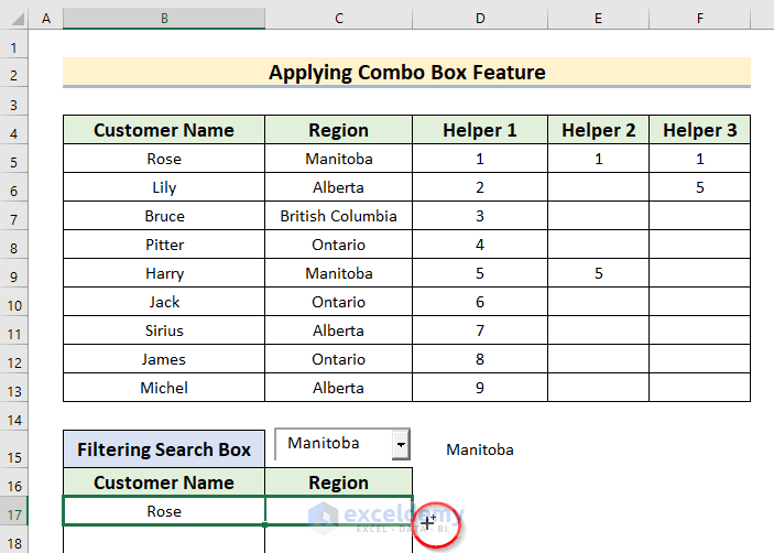
- Drag the mouse pointer up to cell B18. You can not use the mouse pointer at once to apply the formula to the rest of the cell; you have to do this cell by cell.
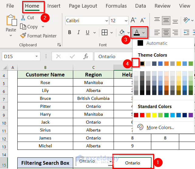
- From the Home tab >> make the font color White in cell D15.
Select any value from the Combo Box to get it along with the related cell values in the table below.
Method 4 – Using the Filter Feature
Steps:
- Select the full range of cells of the dataset.
- Go to the Data tab in the top ribbon.
- Cclick on the Sort & Filter options and select the Filter Feature.
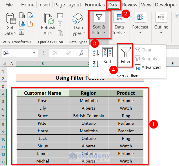
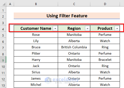
- As a result, you will see the dataset will turn into a table and there will be a Filter arrow icon in the Header cells.
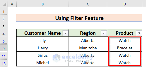
- Click on the Filter icon in the Product header cell.
- You will see some options open.
- Mark the items that you want to show and unmark the items that you want to hide in the list.
- Press OK.
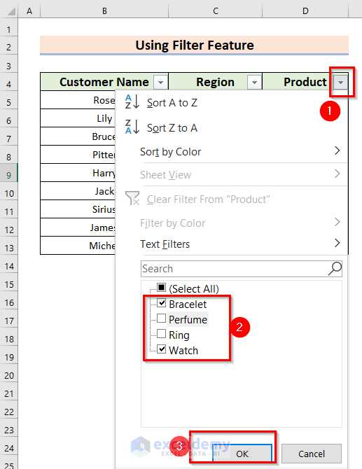
- As a result, you will see only the marked items in the dataset. And, the unmarked item rows have become hidden. You can use the Filter feature to search specific items.
Method 5 – Using the Text Box Feature
Steps:
- Make a table for your data. To do this, follow the first portion of method 2.
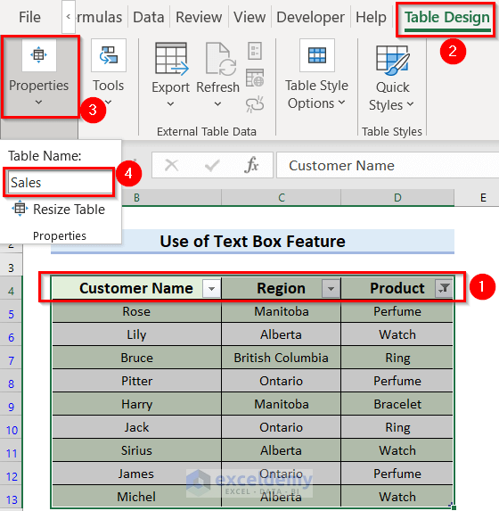
- Select the header cells of the data table.
- Go to Table Design in the top ribbon.
- Select the Properties menu and insert Table Name as Sales.
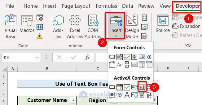
- Go to the Developer tab >> click on the Insert option.
- Select the Text Box option in the ActiveX Controls section.
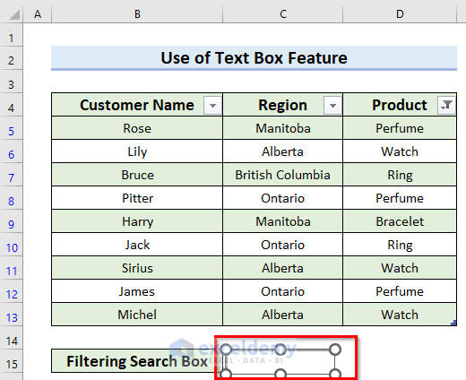
- Draw a Text Box by dragging the mouse pointer in a suitable position as of your need.
- Right-click on the newly created Text Box to open the Context Menu Bar.
- From the Context Menu Bar >> select the Properties option.
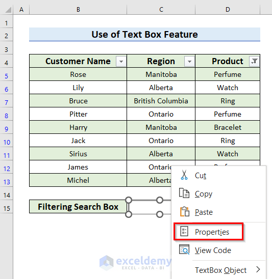
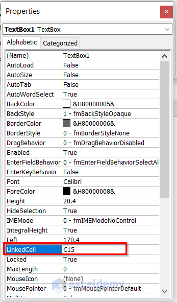
A window named Properties will appear.
- Find the LinkedCell box option and insert C15 in the box.
- Close this window.
- Double-click on the Text Box to open the VBA section.
- Enter the following code in between Private Sub and End Sub.
Private Sub TextBox1_Change()
Application.ScreenUpdating = False
ActiveSheet.ListObjects("Sales").Range.AutoFilter Field:=3, Criteria1:=[C15] & "*", Operator:=xlFilterValues
Application.ScreenUpdating = True
End Sub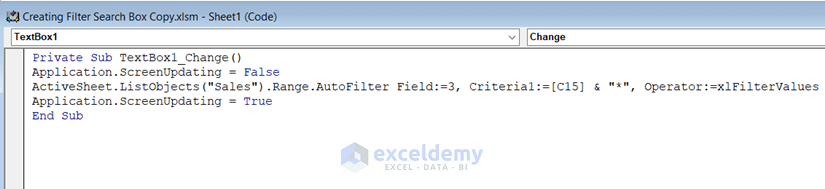
Code Breakdown
- Here, Sales is the array or data table.
- AutoFilter Field:=3 —> denotes based on which cell filter will be working. Here, I have used Field 3 for filtering, which is the 3rd column of your given table. Thus, Field 3 denotes the Product column of the table.
- Criteria1:=[C15] —> denotes that whatever you search that value you will see in the C15 cell.
- Minimize the VBA code.
- Select the Text Box.
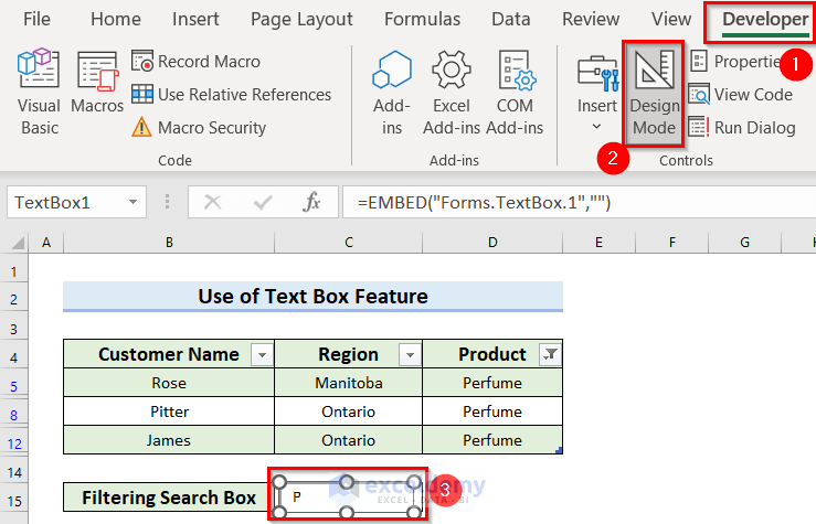
- From the Developer tab >> uncheck the Design Mode option.
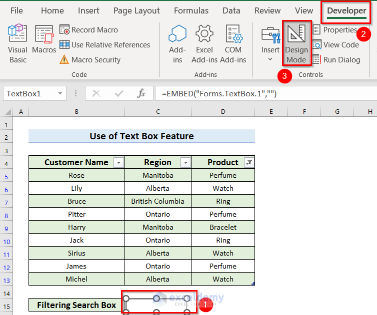
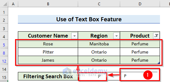
When I have written P in the Text Box, the cell C15 value will also be P. It will filter the data for the Product whose name starts with P. In the case of no matched product, it will remain blank.
- From the Developer tab >> select the Design Mode option.
- Select the Text Box. Drag this to cell C15.
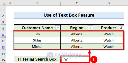
You can see that when I write W in the Text Box, it filters the corresponding data for the Product whose name starts with W.
Read More: Create a Search Box in Excel with VBA
Method 6 – Using Conditional Formatting
Steps:
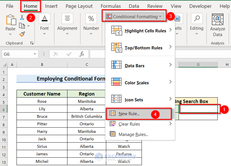
- Select the cell where you want to keep the filtering search box. Don’t select any cell below your Excel data. If you do, then the formula might not work. I have selected cell G6.
- From the Home tab >> go to the Conditional Formatting command.
- Choose the New Rule option to apply the formula.
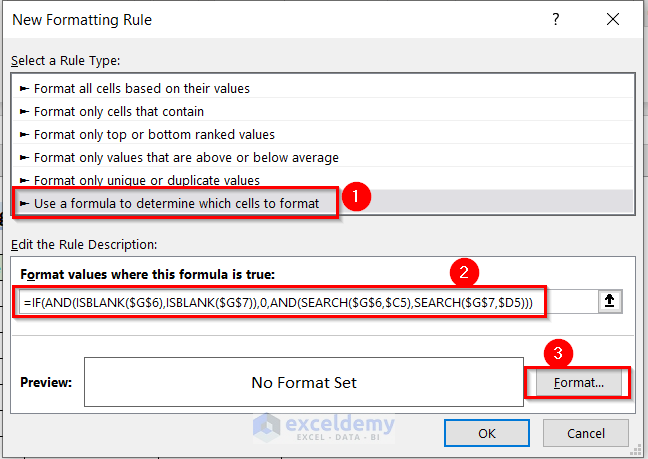
A dialog box named New Formatting Rule will appear.
- From that dialog box, select Use a formula to determine which cells to format.
- Enter the following formula in the Format values where this formula is true: box.
=IF(AND(ISBLANK($G$6),ISBLANK($G$7)),0,AND(SEARCH($G$6,$C5),SEARCH($G$7,$D5)))- Go to the Format menu.
Formula Breakdown
- The ISBLANK function will check whether the cell is empty.
- The AND function will join multiple logics.
- The IF function will test whether both cells G6 and G7 are empty. If they are empty, it will return 0; otherwise, the SEARCH function will work. Here, the Dollar($) sign denotes the fixed cells.
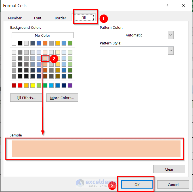
A dialog box named Format Cells will appear.
- From the Fill option >> choose any of the colors. Here, I have chosen Orange, Accent 2, and Lighter 60%. Choose a light color because dark colosr may hide the input data.
- Press OK to apply the formation.
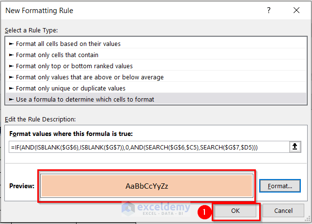
- Press OK on the New Formatting Rule dialog box. Here, you can see the sample instantly in the Preview box.
- From the Home tab >> go to the Conditional Formatting command.
- Choose the Manage Rules option.
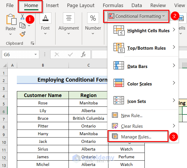
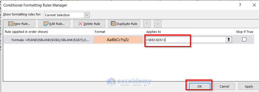
A new window named Conditional Formatting Rules Manager will appear.
- In the Applies to box, select the whole data range. Here, I have selected the range B5:D13.
- Press OK to get the changes.
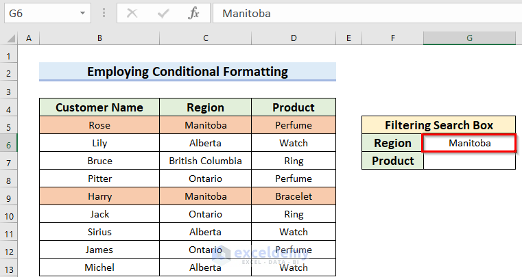
Now, if you write down any region in the Region box, you will get all the corresponding data as highlighted.
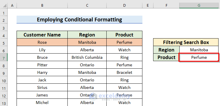
If you also specify the Product name, then it will highlight the cells according to both that particular region and product.
Read more: How to Create Search Box in Excel with Conditional Formatting
Things to Remember
- Here, method 1(Data Validation), method 3 (Combo Box), and method 4(Filter Feature) both have a drop-down arrow as a filtering search box. So, you don’t need to write anything to get filtered data. You can choose your wanted name or ID for the corresponding data.
- In the case of method 2(Combined Functions) and method 5(Text Box), you can get the filtered data by typing just a letter.
Download the Practice Workbook
You can download the practice workbook from here:
Related Articles
- How to Create a Search Box in Excel Without VBA
- How to Create a Search Box in Excel for Multiple Sheets
<< Go Back to Search Box in Excel | Data Management in Excel | Learn Excel
Get FREE Advanced Excel Exercises with Solutions!
