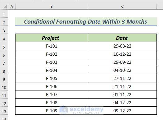
The following dataset has Project and Date columns. In the Date column, 29-08-22 is the first date, and all other dates are ahead of 29-08-222.
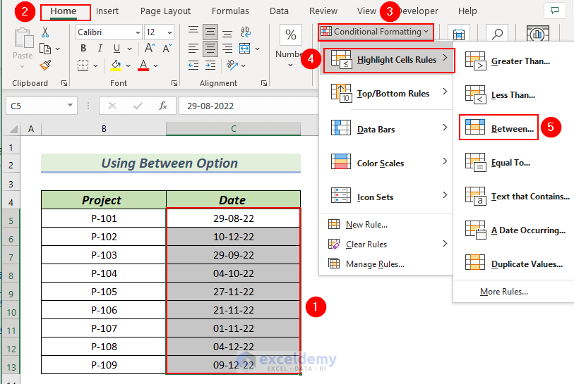
Method 1 – Using the Between Option of Conditional Formatting
Steps:
- Select C5:C13.
- Go to the Home tab >> select Conditional Formatting.
- In Highlight Cells Rules >> select Between.
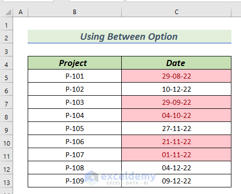
In the Between dialog box:
- Set a range between 24-08-22 and 24-11-22.
- Set Light Red Fill with Dark Red Text as the color.
- Click OK.

You will see dates within 3 months highlighted with light red color.
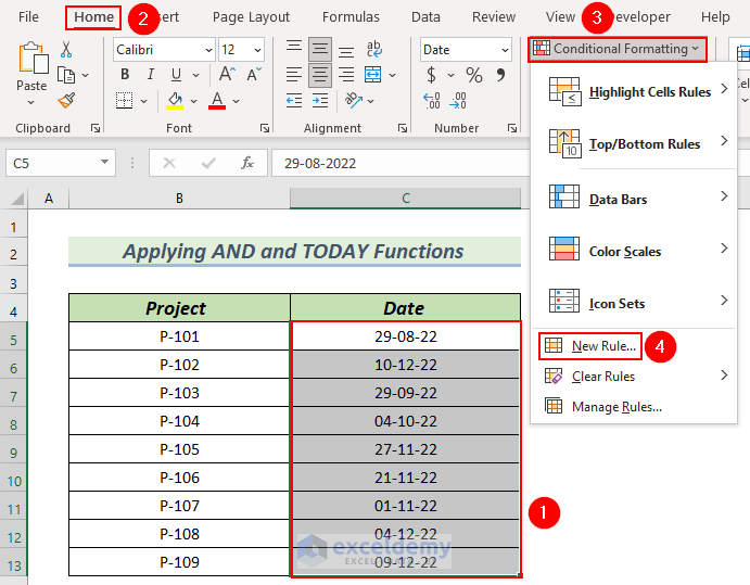
Method 2 – Conditional Formatting a Date Within 3 Months Using the AND and TODAY Functions
Steps:
- Select C5:C13.
- Go to the Home tab >> select Conditional Formatting.
- Select New Rule.
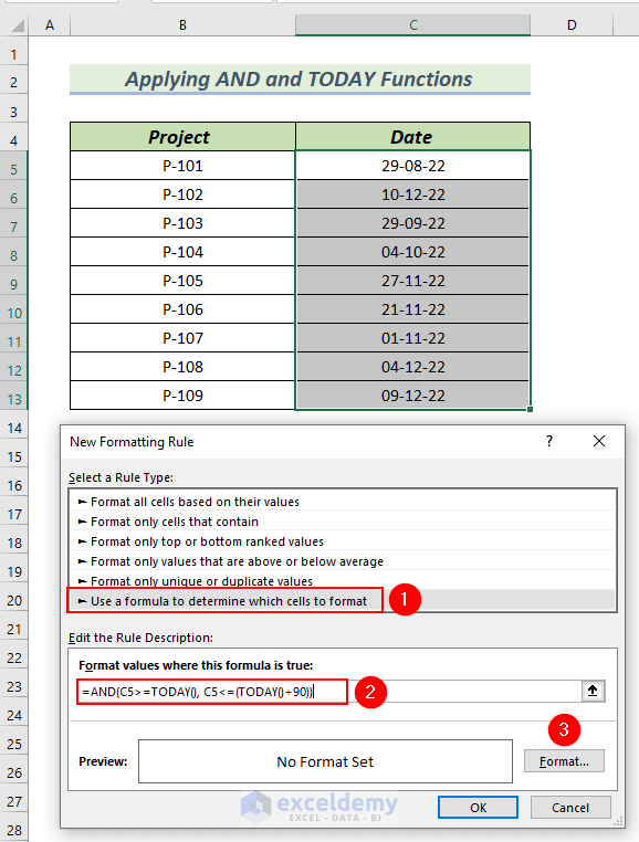
In the New Formatting Rule dialog box:
- Select Use a formula to determine which cells to format in Select a Rule Type.
- Enter the following formula in Format values where this formula is true.
=AND(C5>=TODAY(), C5<=(TODAY()+90))the AND function has two logical conditions for the date range: the Date has to be greater than or equal to today and less than or equal to TODAY()+90. The TODAY function returns the current date. If conditions are fulfilled, dates will Fill Blue.
- Click Format.
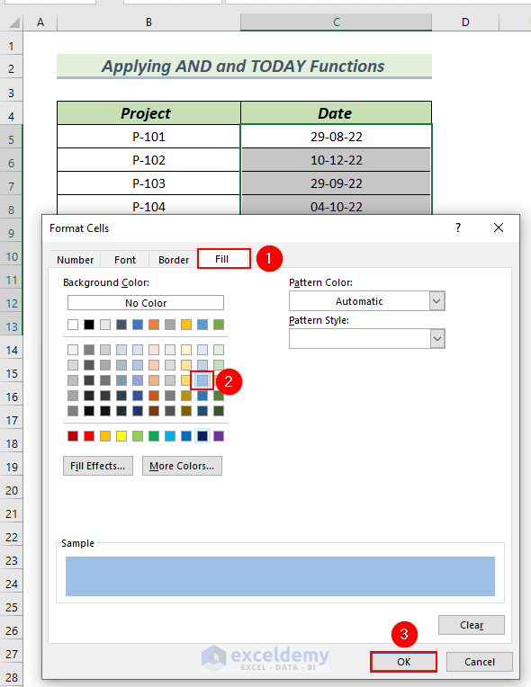
In the Format Cells dialog box:
- In Fill >> select Blue.
- Click OK.
You can see the Preview in the New Formatting Rule dialog box.
- Click OK.
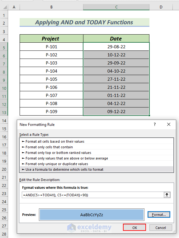
Dates within 3 months are highlighted with blue color.
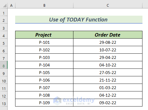
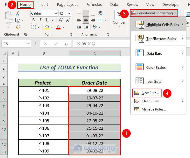
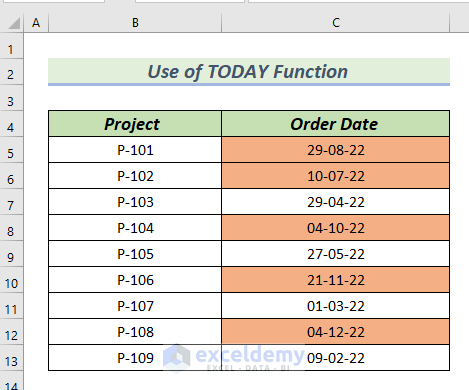
Method 3 – Using the TODAY Function to apply Conditional Formatting to a Date Within 3 Months
In the following dataset the Order Date includes dates that are behind 29-08-22. There are also dates ahead of 29-08-22.
Steps:
- Select C5:C13.
- Go to the Home tab >> select Conditional Formatting.
- Select New Rule.
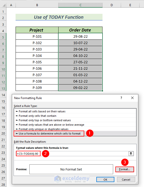
The New Formatting Rule dialog box will be displayed.
- Select Use a formula to determine which cells to format in Select a Rule Type.
- Enter the following formula in Format values where this formula is true.
=C5>TODAY()-90- Click Format.
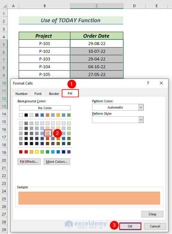
In the Format Cells dialog box:
- In Fill >> select light Orange.
- Click OK.
You can see the Preview in the New Formatting Rule dialog box.
- Click OK.
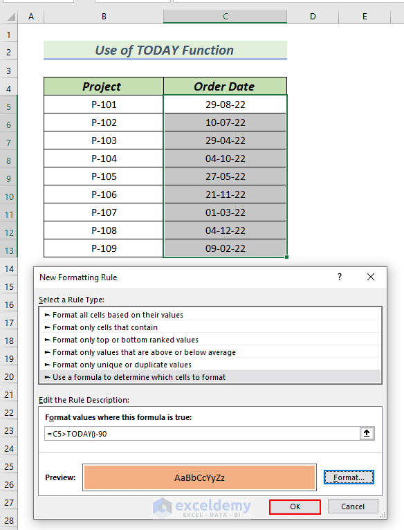
Dates 3 months after and before today are highlighted with light Orange color.
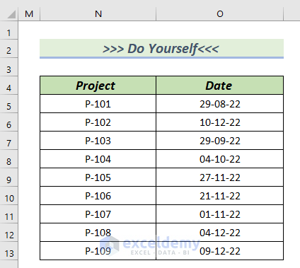
Practice Section
Download the Excel file to practice.
Download Practice Workbook
Download the Excel file and practice.
<< Go Back to Dates | Compare | Learn Excel
Get FREE Advanced Excel Exercises with Solutions!
