This is an overview.
Character codes depend on the Font.
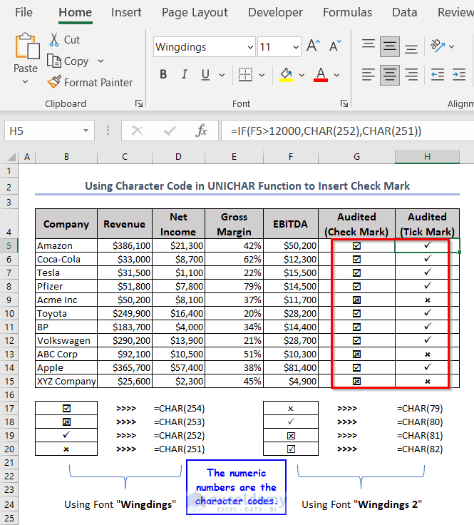
In Wingdings, the character code for the check mark is 252 and the character code for check mark inside a box is 254.
Example 1 – Using the Character Code in Excel Functions to Insert a Check Mark
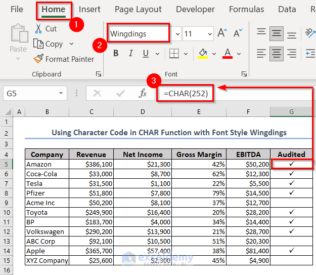
1.1 Using the CHAR Function with the Wingdings Font
- Select the range >> Home tab >>Font group >> change the font to Wingdings.
- Select a cell to use the check mark >> enter the following formula:
=CHAR(252)- Press ENTER.
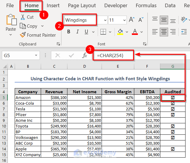
Use another character code as argument in the CHAR function to get the check mark in a box.
- Set the font to Wingdings.
- Select a cell to use the check mark >> enter the following formula.
=CHAR(254)- Press ENTER.
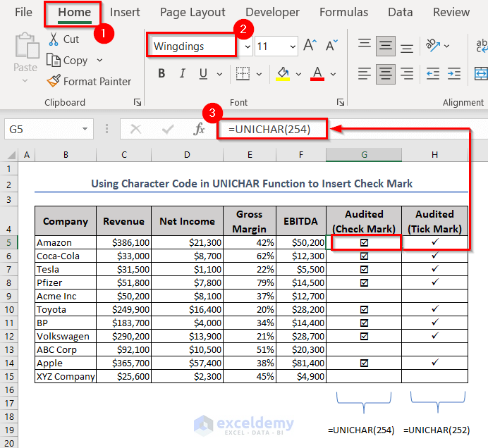
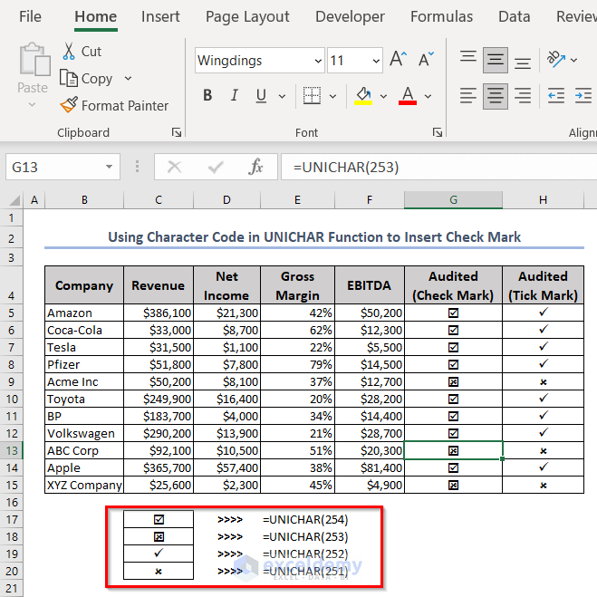
1.2 Applying the UNICHAR Function
- Select the cell range >> Home tab >> Font >> change the font to Wingdings.
- Select a cell to use the check mark >> enter the following formula:
=UNICHAR(254)- Press ENTER.
You can also use UNICHAR(252) to insert a check mark.
1.3 Character Code for a Cross Symbol
- The character code 251 in Wingdings denotes the cross symbol and character code 253 returns the cross symbol in a box.
1.4 Using the Character Code to Create an Excel Formula
To check if a company has more than $12000 EBITDA :
- Use the following formula:
=IF(F5>12000,CHAR(254),CHAR(253))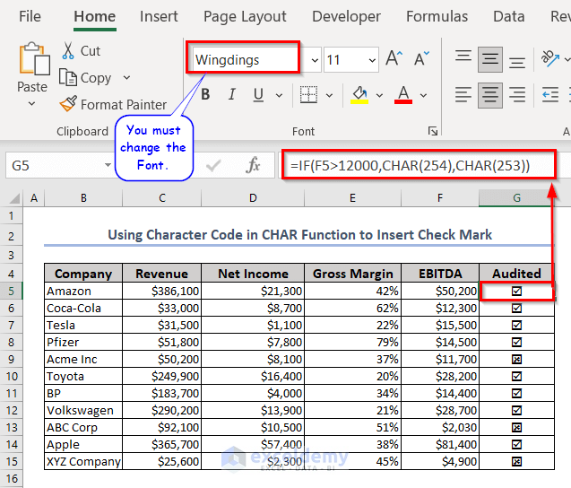
Formula Breakdown
- the IF function checks whether the value in F5 is greater than 12000.
- If the value is greater than 12000, it returns CHAR(254).
- CHAR(254) is the check mark inside the box.
- Otherwise, the IF function returns CHAR(253): a cross inside the box.
- Drag down the Fill Handle to see the result in the rest of the cells.
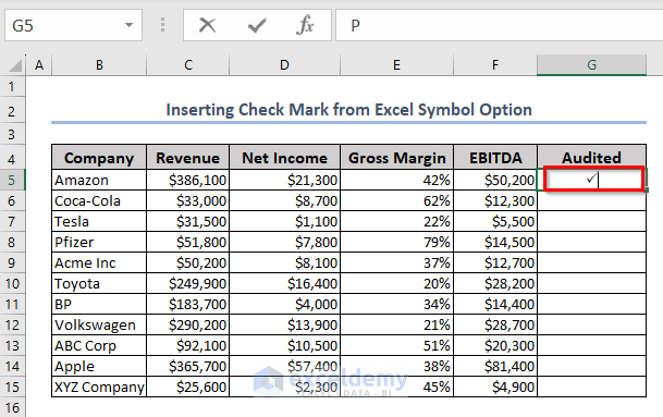
Example 2 – Inserting a Check Mark in the Excel Symbol Option
- Select the cell to insert the check mark.
- In the Insert tab >> go to Symbols >> choose Symbol.
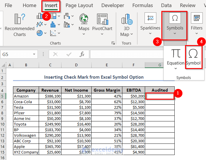
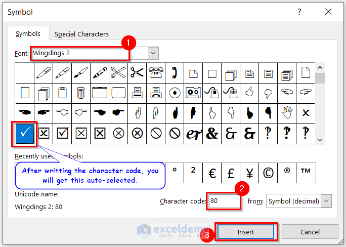
In the Symbol dialog box:
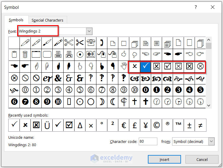
- In Font >> select Wingdings 2 >> in Character code >>enter 80 (the check mark is selected).
- Click Insert.
This is the output.
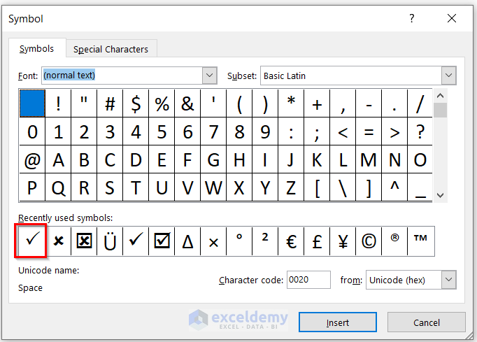
- To use this symbol again, go to Insert tab >> Symbols >> choose Symbol.
- In the Symbol dialog box, you will see the Recently used symbols >> select check mark >> click Insert.
In Wingdings 2, you can use character codes from 79 to 86:
- 79 —> cross symbol.
- 80 —> check mark.
- 81 —> cross inside a box.
- 82 —> check mark inside a box.
- 83 —> a straight cross inside a box.
- 84 —> a bold straight cross inside a box.
- 85 —> a cross inside a circle.
- 86 —> a bold cross inside a circle.
In Wingdings, you can use the character codes from 251 to 254:
- 251 —> cross symbol.
- 252 —> check mark.
- 253 —> cross inside box.
- 254 —> check mark inside a box.

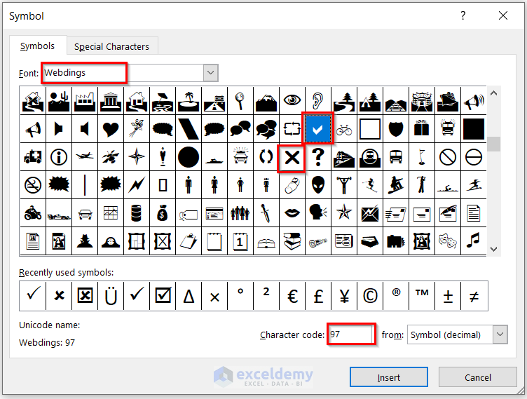
In Webdings:
- 97 —> check mark.
- 114 —> cross mark.
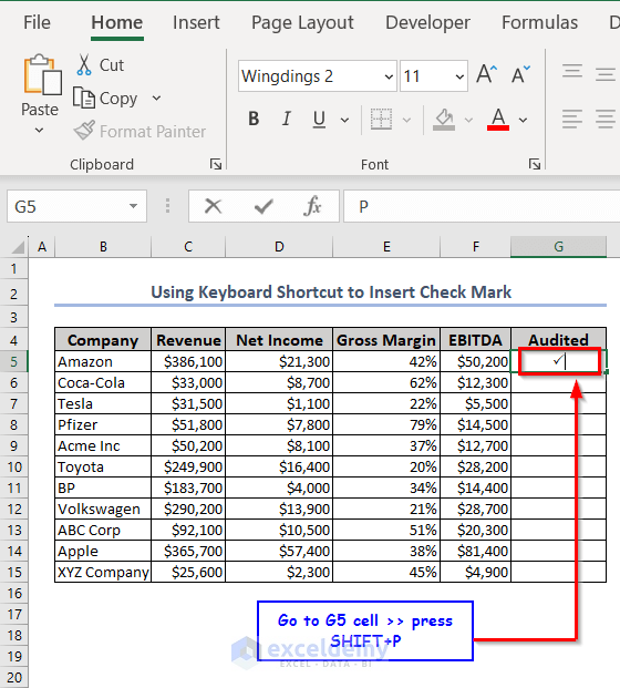
Example 3 – Using Keyboard Shortcuts Based on the Character Codes
- Select G5:G15 >> Home >> Font >> Font drop-down >> Wingdings 2.
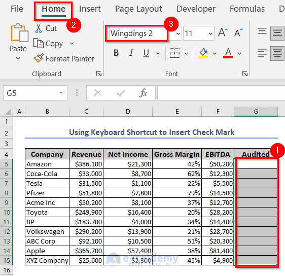
- Select G5 >> press SHIFT+P to get the check mark.
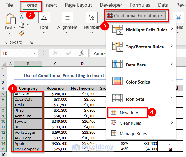
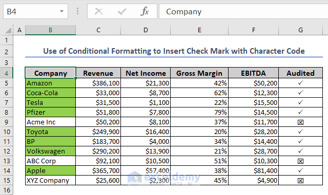
Example 4 – Use Conditional Formatting to Highlight the Check Mark
To highlight the audited companies.
- Select the range to highlight >>go to the Home tab >> Conditional Formatting >> click New Rule.
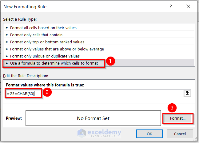
- In New Formatting Rule, select Use a formula to determine which cells to format.
- Enter the following formula in Format values where this formula is true:
=G5=CHAR(80)The Logical Test checks whether the value in G5 is equal to CHAR(80). If the value in G5 is equal to CHAR(80), it will color B5. Otherwise, it remains with No color.
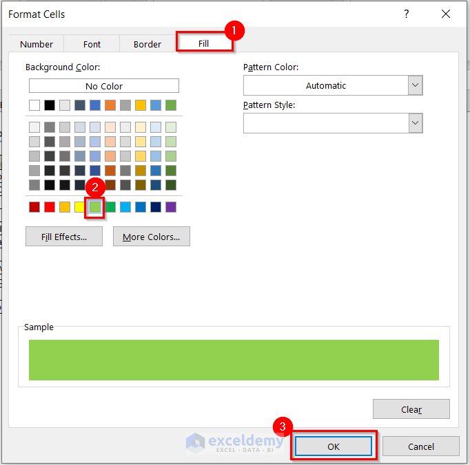
- Go to Format.
- In Format Cells, select Fill.
- Choose a color. Here, Light Green.
- Click OK.
- Click OK in the New Formatting Rule dialog box.
This is the output.
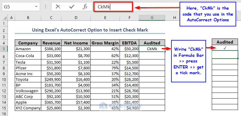
Example 5 – Using the Excel AutoCorrect Options to Create a Customized Character Code and Include a Check Mark
- Go to File >> click Options.

In the Excel Options dialog box:
- In Proofing >> click AutoCorrect Options >> AutoCorrect: English (United States).
- Enter a value for the check mark in Replace >> copy a check mark (✓) and enter it in With >> Click OK.
- Click OK in Excel Options.

“CkMk” was entered as the code for the check mark.
- Enter “CkMk” in the Formula Bar >> press ENTER >> get a check mark instead of “CkMk“.
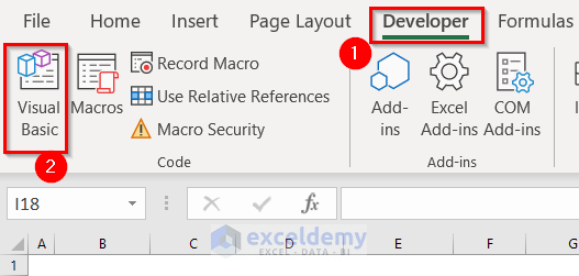
How to Insert a Check Mark Without a Character Code in Excel Using a VBA Macro
- Open the Visual Basic Editor, in the Developer tab >> go to Visual Basic.
1. Add a Check Mark in a Cell or Range of Cells Based on a Selection
- In the Insert tab >> select Module >> enter the following code.
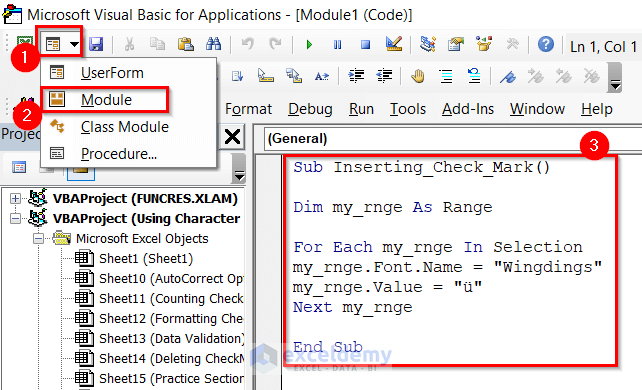
Sub Inserting_Check_Mark()
Dim my_rnge As Range
For Each my_rnge In Selection
my_rnge.Font.Name = "Wingdings"
my_rnge.Value = "ü"
Next my_rnge
End Sub
Code Breakdown:
- The variable my_rnge is declared as Range.
- A For Each loop calls every cell in the range.
- The .Font property changes the font to Wingdings and the .Value property enters the cell value to ü.
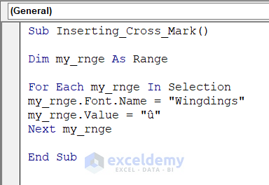
- Insert another module >> Enter the following code in Module2.
Sub Inserting_Cross_Mark()
Dim my_rnge As Range
For Each my_rnge In Selection
my_rnge.Font.Name = "Wingdings"
my_rnge.Value = "û"
Next my_rnge
End Sub
This code is similar to the previous one, but the cell value is û.
- Save the codes >> go back to the Excel sheet.
- In the Developer tab >> go to Insert >> choose Form Controls >> drag a Button.
- In the Assign Macro dialog box >> select the macro: Inserting_Check_Mark >> click OK.
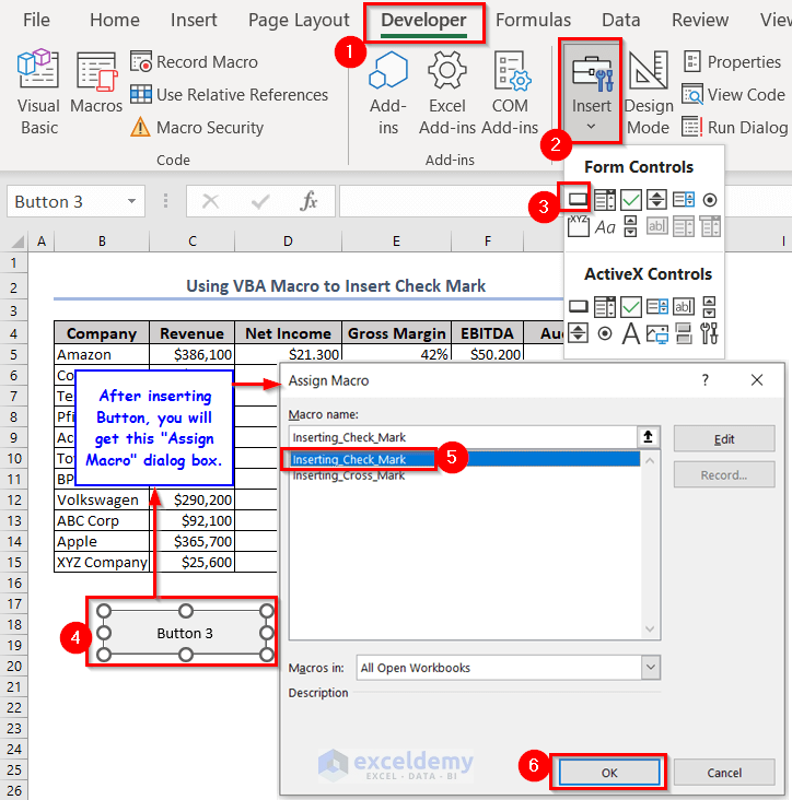
- Insert another button >> assign it to the macro: Inserting_Cross_Mark.
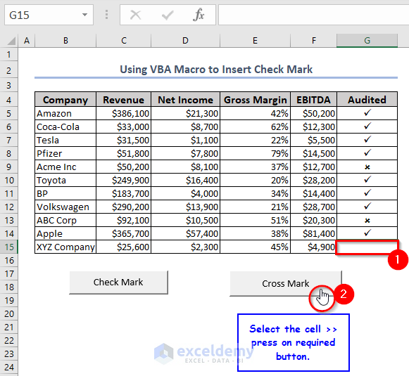
If you press the Inserting_Check_Mark button, you will get a check mark. If you press the Inserting_Cross_Mark button, you will get a cross mark.
- Right-click the buttons >> click Edit Text >> change the names.
- Go to a cell and press a button to see the symbol.
Read More: How to Add Characters in Excel
2. Double Click the Cell to Add a Check Mark in Excel
- Right-click the sheet name (VBA Macro-2) to go to the Context Menu Bar >>select VBA Code.
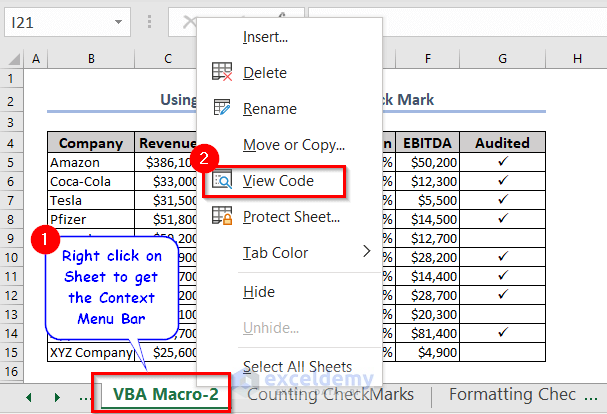
- In the Visual Basic Editor, enter the following code:
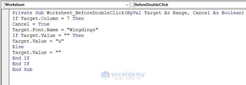
Private Sub Worksheet_BeforeDoubleClick(ByVal Target As Range, Cancel As Boolean)
If Target.Column = 7 Then
Cancel = True
Target.Font.Name = "Wingdings"
If Target.Value = "" Then
Target.Value = "ü"
Else
Target.Value = ""
End If
End If
End Sub- Double-clicking G7 will insert a check mark.
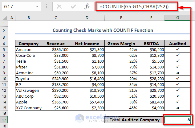
How to Count Check Marks in Excel
- To count the check marks, use the following formula.
=COUNTIF(G5:G15,CHAR(252))The COUNTIF function counts all the cells containing CHAR(252) or a check mark.
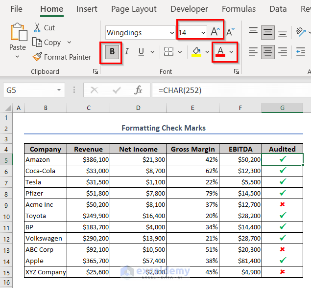
How to Format Check Marks in Excel
You can increase/ decrease the Font Size, change the Font Color, make them Bold or Italic, and Underline check marks.
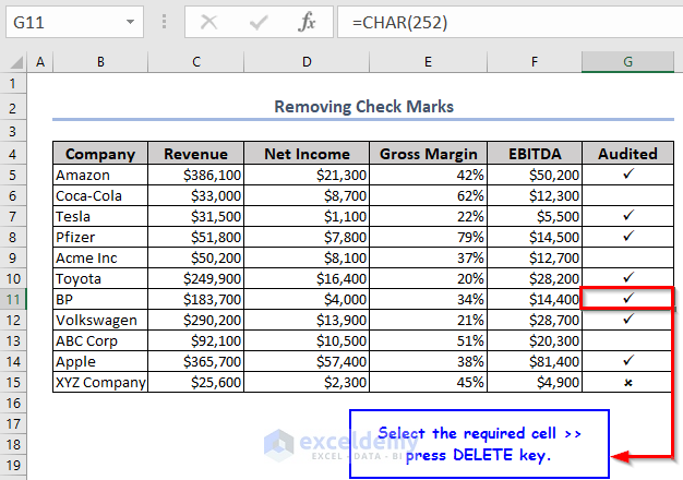
How to Remove Check Marks in Excel
- Select the cell >> Press DELETE.
The check mark is removed.
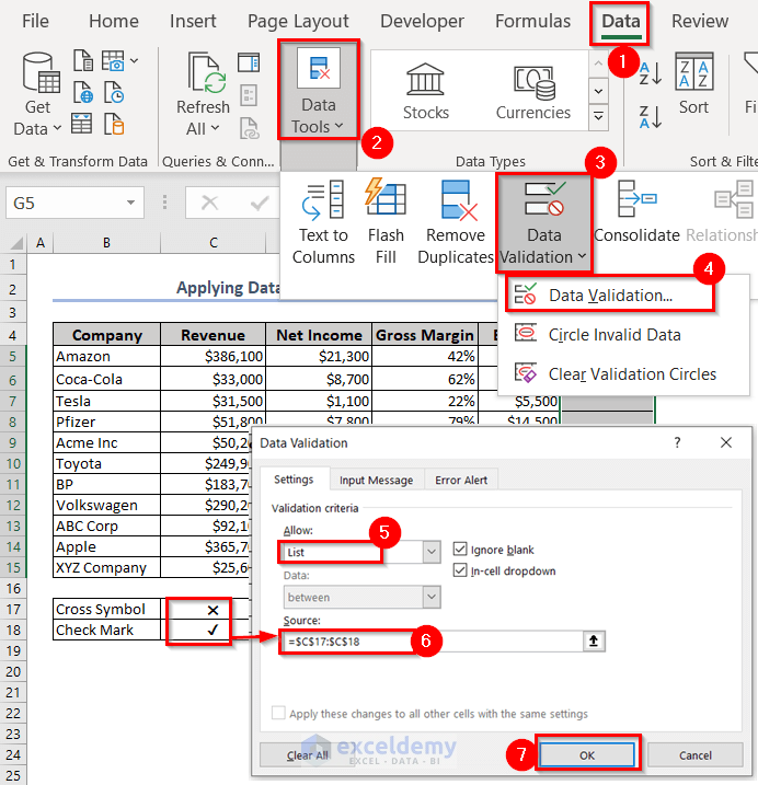
Using Check Marks as Symbols in Excel
- Copy the check mark and the cross symbol and paste them in the Excel sheet.
- Select G5:G15 to use the check marks.
- Go to the Data tab >> Data Tools >> Data Validation >> select Data Validation.
- In Allow>> choose List >> in Source >> enter C17:C18 >> click OK.
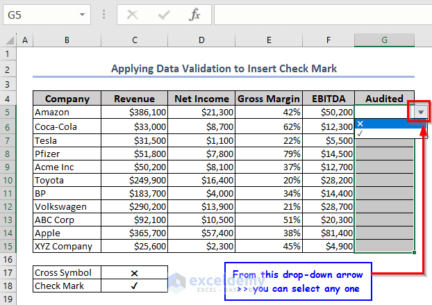
- You will see a drop-down arrow in every cell of the selected range. Click the drop-down arrow and select a symbol.
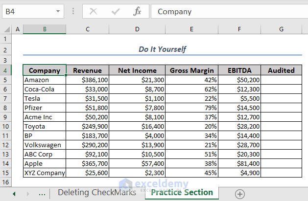
Practice Section
Practice here.
Download Practice Workbook
Download the practice workbook.
Frequently Asked Questions
1. Check Mark Vs Check Box in Excel
A check mark is just a symbol.A check box is a blank box.
2. How to insert a checkbox in Excel?
Go to the Developer tab >> Insert >> Form Controls >> Check Box (Form Control).
3. How to Insert a Check Mark Symbol in Word?
In the Insert tab of Microsoft Word >> Symbols >> Symbol >> More Symbols >> Symbol dialog box >> Font Wingdings and Character code 252 >> Insert.
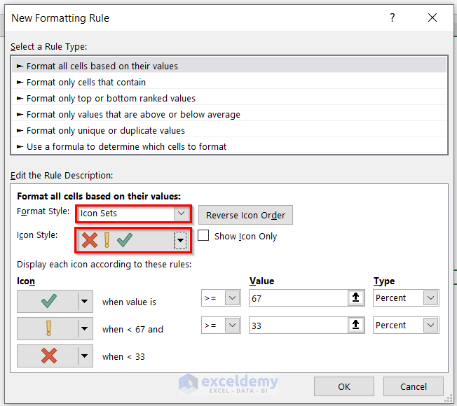
4. Is there a way to get a check mark in Conditional Formatting?
Yes. In Conditional Formatting >> go to New Rule >> choose Icon Sets in Format Style >> select Icon Style as Cross-Check.
<< Go Back to Learn Excel
Get FREE Advanced Excel Exercises with Solutions!
