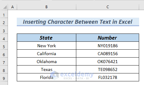
The following dataset has the State and Number columns. Using this dataset, we will demonstrate how to insert characters between text in Excel.
Method 1 – Use the LEFT and MID Functions with the Ampersand Operator
In the Number column, we want to add a Hyphen(–) between the state abbreviation and numbers.
- Copy the following formula in the result cell D5:
=LEFT(C5,2) & "-" & MID(C5,3,100)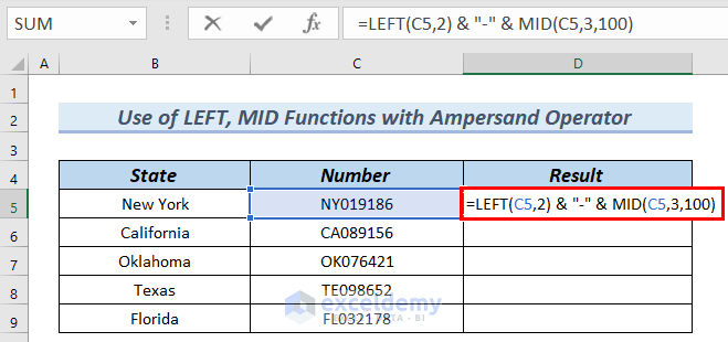
Formula Breakdown
- LEFT(C5,2) → the LEFT function returns the character or characters from the beginning position in a number or text string of a cell. The returned characters are based on the number we specify.
- LEFT(C5,2) → becomes
- Output: NY
- MID(C5,3,100) → the MID function returns characters from a text string. It begins from the position we specify and returns the number of characters that we specify.
- MID(C5,3,100) → becomes
- Output: 019186
- NY& “-” &019186 → the Ampersand operator connects NY with Hyphen (-) and 019186.
- NY& “-” &019186 → becomes
- Output: NY-019186
- Explanation: a Hyphen (–) is added between the abbreviation NY and the numbers 019186 in cell D5.
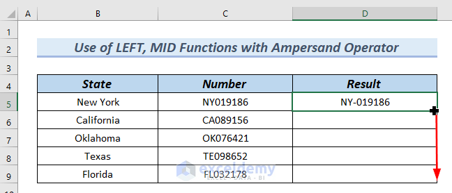
- Press Enter. You can see the result in cell D5.
- Drag down the formula with the Fill Handle tool.
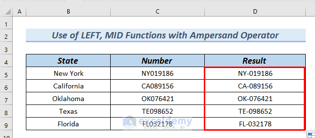
- In the Result column, you can see the inserted character between text.
Read More: How to Add Characters in Excel
Method 2 – Applying the REPLACE Function to Insert a Character Between Text
We will add a number code (+889) between the state abbreviation and the numbers of the Number column.
- Copy the following formula in cell D5.
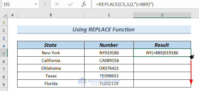
=REPLACE(C5,3,0,"(+889)")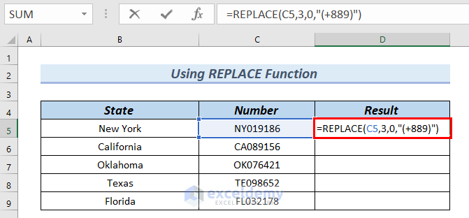
Formula Breakdown
- REPLACE(C5,3,0,”(+889)”) → the REPLACE function replaces a portion in the text string with another number or text we specify.
- REPLACE(C5,3,0,”(+889)”) → becomes
- Output: NY(+889)019186
- Explanation: here, (+889) is added between NY and the numbers 019186 in cell D5.
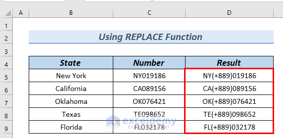
- Press Enter.
- Drag down the formula with the Fill Handle tool.
- You can see the inserted character between text in all cells.
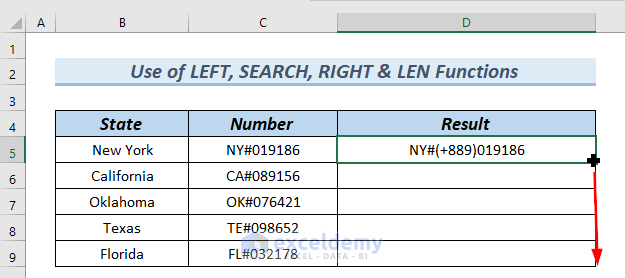
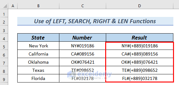
Method 3 – Using the LEFT, SEARCH, RIGHT, and LEN Functions
In the following dataset, you can see in the Number column that there is a Hash (#) sign between the state abbreviation and numbers. We will add a number code (+889) after the Hash (#) sign.
- Insert the following formula in cell D5.
=LEFT(C5, SEARCH("#", C5)) &"(+889)"& RIGHT(C5, LEN(C5) - SEARCH("#", C5))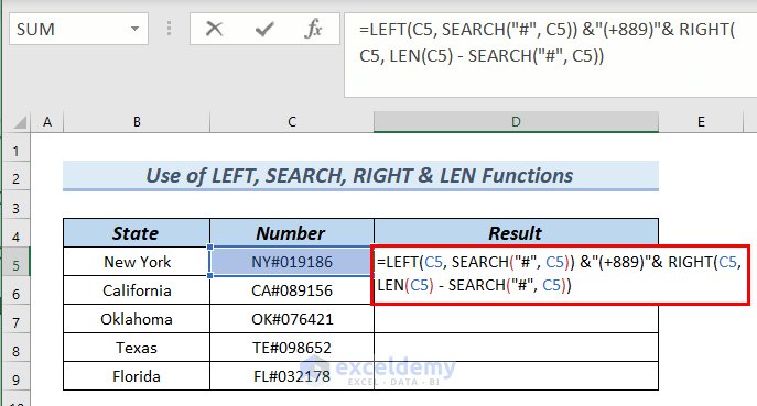
Formula Breakdown
- SEARCH(“#”, C5) → the SEARCH function returns the number of characters at which a specific character or text string is first found, reading from left to right. Here, the SEARCH function finds out the position of the Hash (#) in cell C5.
- Output: 3
- LEN(C5) → the LEN function returns the total number of characters in cell C5.
- Output: 9
- RIGHT(C5, LEN(C5) – SEARCH(“#”, C5)) → the RIGHT function returns the character or characters from the end position in a number or text string of a cell. The returned characters are based on the number we specify.
- RIGHT(C5, 9- 3) → becomes
- Output: 019186
- SEARCH(“#”, C5)) &”(+889)”& RIGHT(C5, LEN(C5) – SEARCH(“#”, C5)) → the Ampersand “&” operator connects 3 with (+889) and 019186.
- 3 &”(+889)”& 019186 → becomes
- Output: 3(+889)019186
- LEFT(C5, SEARCH(“#”, C5)) &”(+889)”& RIGHT(C5, LEN(C5) – SEARCH(“#”, C5)) → the LEFT function returns the character or characters from the beginning position in a number or text string of a cell. The returned characters are based on the number we specify.
- LEFT(C5,3(+889)019186) → As a result, it becomes
- Output: NY#(+889)019186
- Explanation: here, (+889) is added between NY# and the numbers 019186 in cell D5.
- Press Enter.
- Drag down the formula with the Fill Handle tool.
- This completes the column.
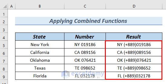
Method 4 – Applying Combined Functions to Insert a Character Between Text
In the following dataset, you can see in the Number column that there is a space (” “) between the state abbreviation and numbers. We will add a number code (+889) after the space (” “).
- Copy the following formula in cell D5.
=CONCATENATE(LEFT(C5, SEARCH(" ", C5)), "(+889)", RIGHT(C5, LEN(C5) -SEARCH(" ", C5)))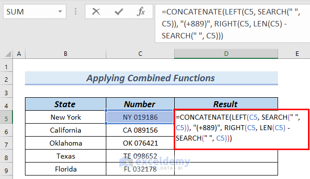
Formula Breakdown
- SEARCH(” “, C5) → the SEARCH function returns the number of characters at which a specific character or text string is first found, reading from left to right. Here, the SEARCH function finds out the position of the space(” “) in cell C5.
- Output: 3
- LEN(C5) → LEN function returns the total number of characters in cell C5.
- Output: 9
- RIGHT(C5, LEN(C5) -SEARCH(” “, C5)) → RIGHT function returns the character or characters from the end position in a number or text string of a cell. The returned characters are based on the number we specify.
- RIGHT(C5, 9-3) → becomes
- Output: 019186
- LEFT(C5, SEARCH(” “, C5))→ LEFT function returns the character or characters from the beginning position in a number or text string of a cell. The returned characters are based on the number we specify.
- LEFT(C5, SEARCH(” “, C5)) → becomes
- Output: NY
- CONCATENATE(LEFT(C5, SEARCH(” “, C5)), “(+889)”, RIGHT(C5, LEN(C5) -SEARCH(” “, C5))) → CONCATENATE function connects or joins the characters into one single text string.
- CONCATENATE(NY , “(+889)”, 019186)) →Then, it becomes
- Output: NY (+889)019186
- Explanation: here, (+889) is added between NY and the numbers 019186 in cell D5.
- Press Enter.
- Drag down the formula with the Fill Handle tool.
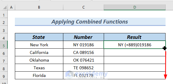
- You can see the inserted character between text in all result cells.
Method 5 – Using VBA to Insert a Character Between Text
- Go to the Developer tab.
- Select Visual Basic.
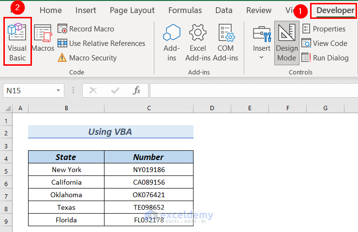
- A VBA editor window will appear.
- From the Insert tab, select Module.
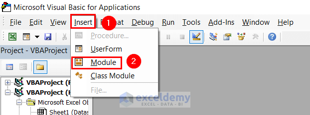
- Next, a VBA Module will appear.
- Copy the following code in the Module.
Sub INSERT_CHARACTER_BETWEEN_CELLS()
Dim Cells As Range
Dim Cell_Range As Range
Set Cell_Range = Application.Selection
Set Cell_Range = Application.InputBox _
("Select Range of Cells to Insert Character", _
"Insert Character Between Cells", Cell_Range.Address, Type:=8)
For Each Cells In Cell_Range
Cells.Value = VBA.Left(Cells.Value, 2) & "(+889)" & _
VBA.Mid(Cells.Value, 3, VBA.Len(Cells.Value) - 1)
Next
End Sub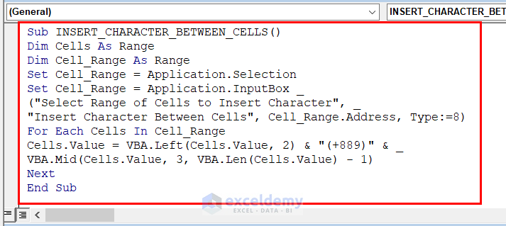
Code Breakdown
- We declare INSERT_CHARACTER_BETWEN_CELLS as our Sub.
- We take Cells and Cells_Range as variables for Range.
- We use the Left, VBA.Mid, and VBA.Len functions for inserting (+889) between selected cells.
- We use the For loop to continue the task unless it finds the last cell.
- Close the VBA editor window.
- Return to the worksheet.
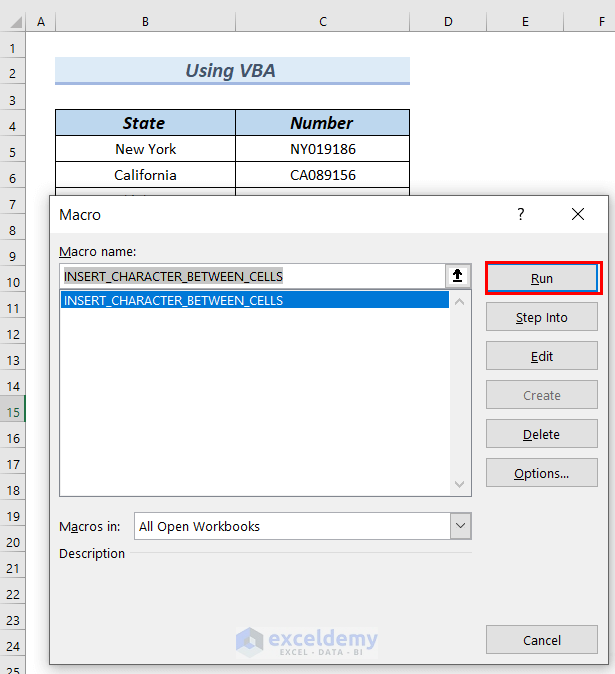
- Press Alt + F8 to bring out the Macro dialog box so that we can run the code.
- At this point, a MACRO dialog box will appear. Make sure the Macro Name contains the Sub of your code.
- Click on Run.
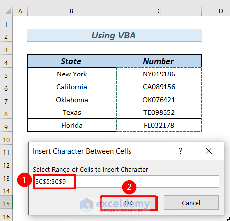
- An Input Box of Insert Character Between Cells will appear.
- In the Select Range of Cells to Insert Character box, select the cells C5:C9.
- Click OK.
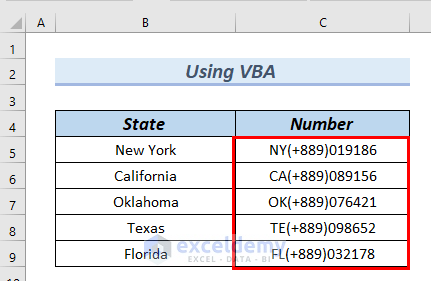
- VBA will input the character into the cells directly.
Practice Section
You can download the Excel file to practice the explained methods.
Download the Practice Workbook
You can download the Excel file and practice while you are reading this article.
<< Go Back to Learn Excel
Get FREE Advanced Excel Exercises with Solutions!

This is good but work only with 2 words in same cell.
do you know to do the same when we have more words in a cell?
Cell A1= john Dole facility open tomorrow
Cell A2= Marcus Miller will start it soon his work
……more cells
Output
A1= john|Dole|facility|open|tomorrow
A2= Marcus|Miller|will|start|soon|his|work|
Thanks
Hello Joe,
You can insert a character between each word in cells with multiple words using Excel’s SUBSTITUTE function combined with TRIM and FIND functions**. Here’s one way to do it:
Replace Each Space with the Character: Use a formula like:
=SUBSTITUTE(A1, ” “, “|”)
This replaces each space in A1 with |, creating the output you’re looking for, e.g., john|Dole|facility|open|tomorrow. Apply this to each cell for consistent results.
Regards
ExcelDemy