Method 1 – Adding a Check Mark with ASCII Characters using the Microsoft Notepad
Steps:
- Open the Microsoft Notepad.
- Press & hold ALT and use the keyboard number pad to enter 251.
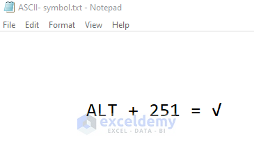
- Copy the check mark and paste it into Microsoft Excel.
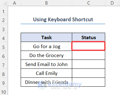
Method 2 – Using Keyboard Shortcuts to Insert a Check Mark
Step 1: Cell Selection
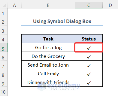
- Select the cells in which you want to insert the check mark. Here, C5.
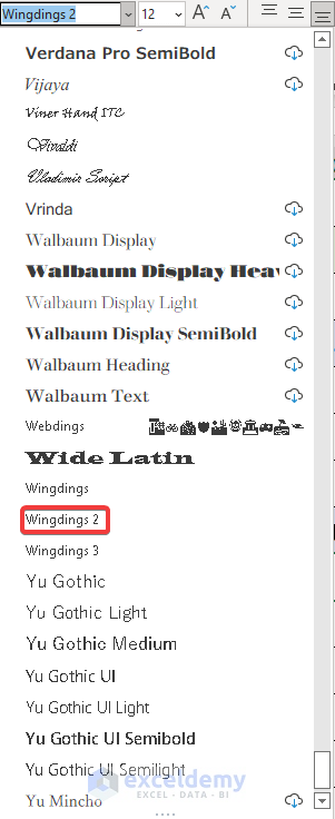
Step 2: Changing the Font
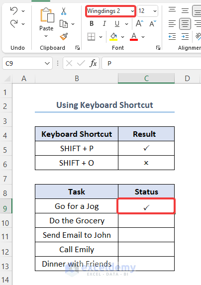
- Change the font to Wingdings 2.
Step 3: Using the Keyboard Shortcuts
- Use, the keyboard shortcuts to insert check and cross marks as shown below.
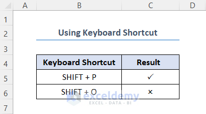
- Press SHIFT + P and ENTER to get a check mark.
- Press SHIFT + O to get a cross mark.
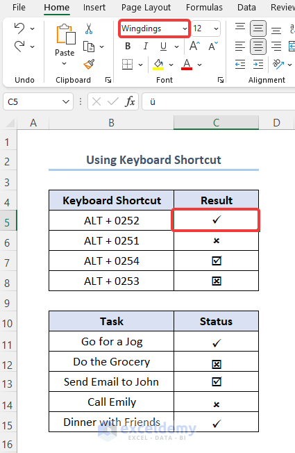
Wingdings can also be used to insert check marks, checkboxes, cross marks & cross boxes.
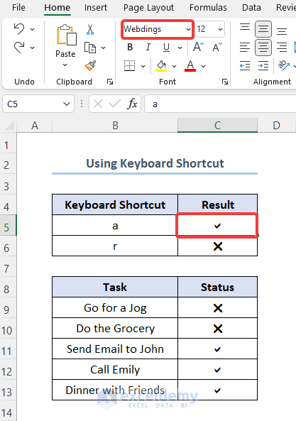
- Webdings can be used to insert check marks & cross marks.
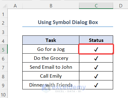
Method 3 – Using the Symbol Dialog Box to Add a check Mark
Step 1: Selecting the Cells
- Here, C5 is selected.

- Go to the Insert tab.
- Select Symbols.
Step 2: Choosing the Font and Character Code
- Click Symbols.
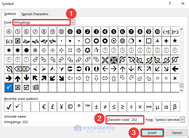
- Change the font to Wingdings.
- Enter 252 in the Character code box and click Insert.
This is the output.
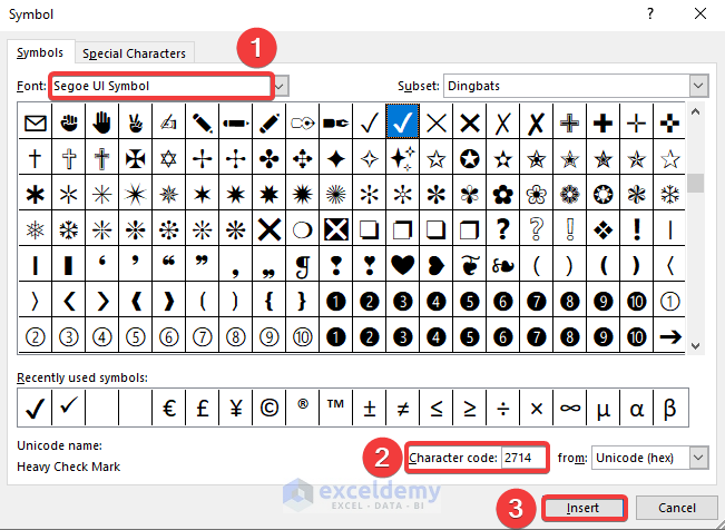
- Copy and paste the symbol. You can also use the Segoe UI Symbol font to get check marks in Excel.
- In the Character code box, enter 2714.
This is the output.
Read More: How to Insert Symbol in Excel Footer
Method 4 – Inserting a check Mark using the Excel CHAR Function
Step 1: Altering the Font
- Select the cell in which you want to insert the check mark. Here, C5.
- Change the font to Wingdings.
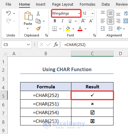
Step 2: Entering the Character Codes
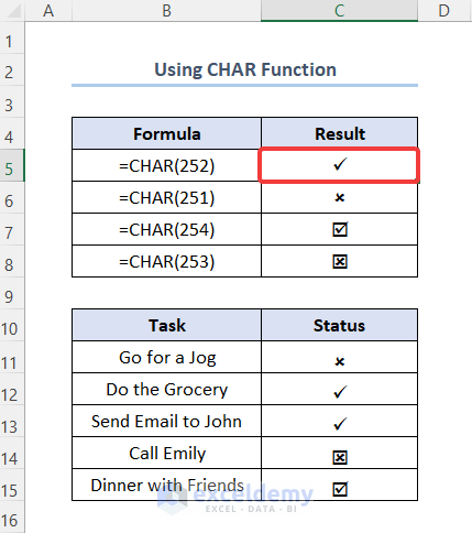
- Enter =CHAR(252) to insert a check mark.
- Insert symbols using the CHAR function based on the codes given in the table below.
Read More: How to Insert Sign in Excel Formula
Method 5 – Using the AutoCorrect Feature to Insert a check Mark
Step 1: Go to the File Tab and Select Options
- Click the File tab.
- Click Options.

Step 2: Proofing and AutoCorrect Options
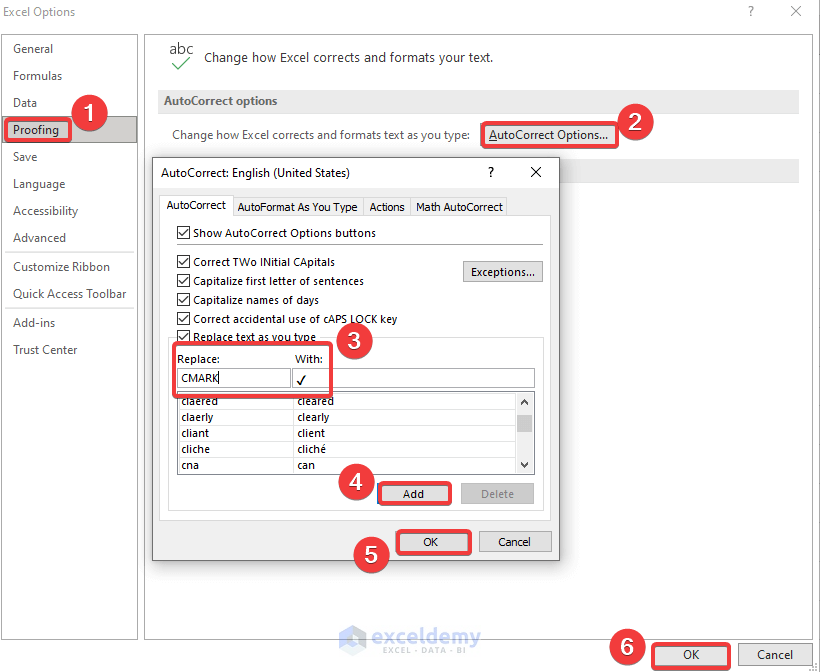
- In Options, select Proofing.
- Click AutoCorrect Options.
- In the dialog box:
- Replace: CMARK
- With: ✔
- Click Add.
- Click OK.
Cells containing CMARK will be replaced with the check mark ✔.
Note:
- The autocorrect feature is case-sensitive. So, CMARK must be in caps.
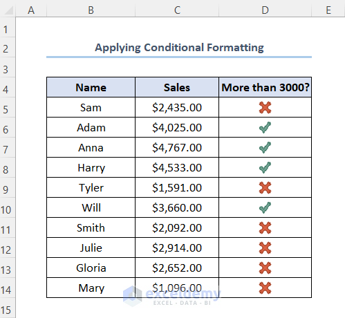
Method 6 – Applying the Conditional Formatting to Insert a check Mark
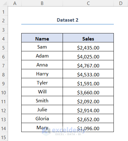
The sample dataset showcases names and their corresponding sales.
To insert a check mark for sales above $3000 and a cross mark for sales below $3000.
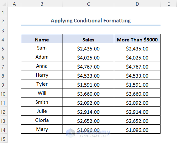
Step 1: Creating a Copy of the Cell
- Enter =C5 in D5. If the values in column C change column D will be updated automatically.
- Drag down the Fill Handle.
Step 2: Using Conditional Formatting
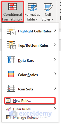
- Select all the cells in the column.
- In the Home tab, click Conditional Formatting.
- Select New Rule.
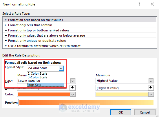
Step 3: Applying a New Rule
- In New Formatting Rule, click Format Style.
- Choose Icon Sets.
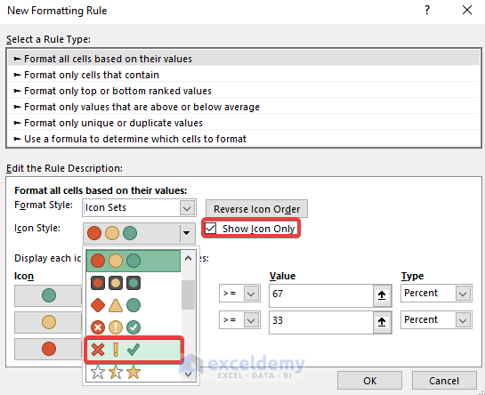
Step 4: Choosing the Icon Sets
- Select the check mark and cross mark.
- Check Show Icon Only.
Step 5: Providing the Condition
- Change the exclamation mark to a cross mark by clicking the dropdown list.
- Change Type from Percent to Number.
- Set the Value and click OK.
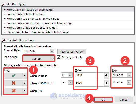
- Insert a check mark for Sales exceeding $3000 and a cross mark for Sales below $3000.
Read More: How to Insert Rupee Symbol in Excel
Method 7 – Using VBA to Add a check Mark
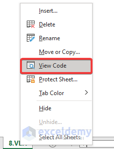
- Right-click the worksheet.
- Click View Code.
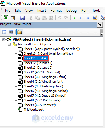
Step 2: Locating the Worksheet
- Select the worksheet from the list.
- Enter the code.
Step 3: Providing the Command
- Press the two dropdowns on the right.
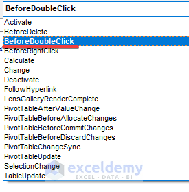
- Click the first dropdown and change it to Worksheet.
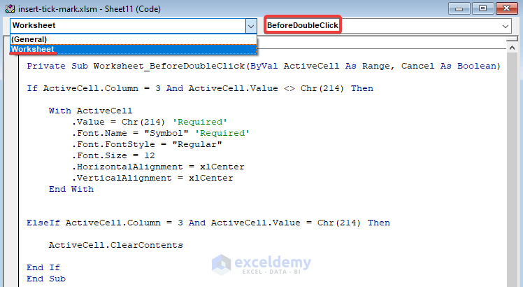
- Click the second dropdown and change it to BeforeDoubleClick.
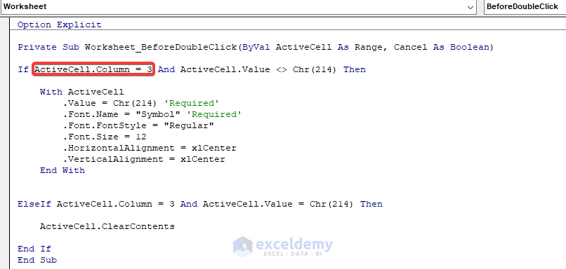
Step 4: Entering the VBA Code
- Copy the code here and paste it.
Option Explicit
Private Sub Worksheet_BeforeDoubleClick(ByVal ActiveCell As Range, Cancel As Boolean)
If ActiveCell.Column = 3 And ActiveCell.Value <> Chr(214) Then
    With ActiveCell
        .Value = Chr(214) 'Required'
        .Font.Name = "Symbol" 'Required'
        .Font.FontStyle = "Regular"
        .Font.Size = 12
        .HorizontalAlignment = xlCenter
        .VerticalAlignment = xlCenter
    End With
ElseIf ActiveCell.Column = 3 And ActiveCell.Value = Chr(214) Then
    ActiveCell.ClearContents
End If
End Sub
The code will insert a check mark in column C (Column = 3).
- Go back to the worksheet.
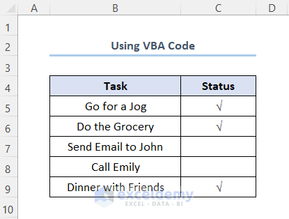
- Double-click the cells to insert a check mark.
- Double-click the cells again to remove it.
Download Practice Workbook
Related Articles
- How to Put Equal Sign in Excel without Formula
- How to Insert Dollar Sign in Excel Formula
- How to Put Sign in Excel Without Formula
- How to Write X Bar in Excel
<< Go Back to Insert Symbol in Excel | Excel Symbols | Learn Excel
Get FREE Advanced Excel Exercises with Solutions!
