Method 1 – Manually Calculating Second Derivative
Steps:
- Select cell C5.
- Enter the following formula:
=2*COS(B5^2)-4*B5*B5*SIN(B5^2)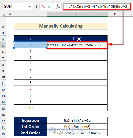
In the formula, we inserted cell B5 as x.
- Press ENTER.
- Drag down the Fill Handle tool to AutoFill the formula for the rest of the cells.
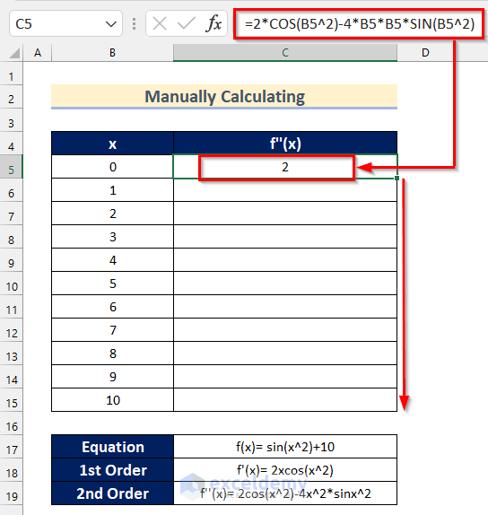
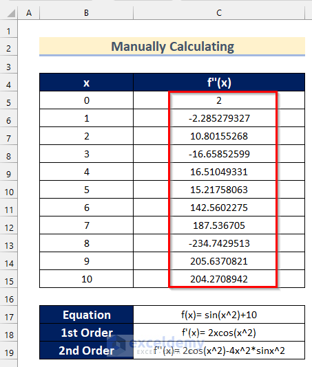
You will calculate all the values of the second derivative of the function manually.
Method 2 – Using Scatter Plot to Calculate 2nd Derivative
Steps:
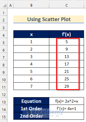
- Select cell C5.
- Enter the following formula:
=4*B5+1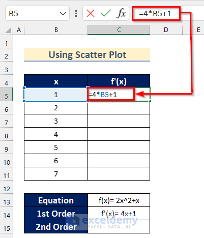
We inserted cell B5 as x.
- Press ENTER.
- Drag down the Fill Handle tool to AutoFill the formula for the rest of the cells.
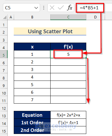
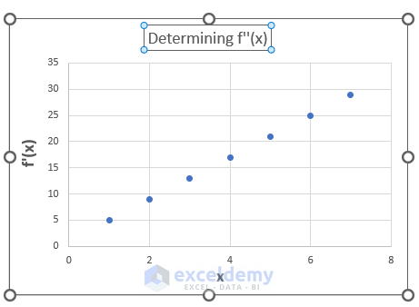
You will get all the values of the first derivative of the function.
- Select cell range B4:C11.
- Go to the Insert tab >> click on Insert Scatter or Bubble Chart >> select Scatter.
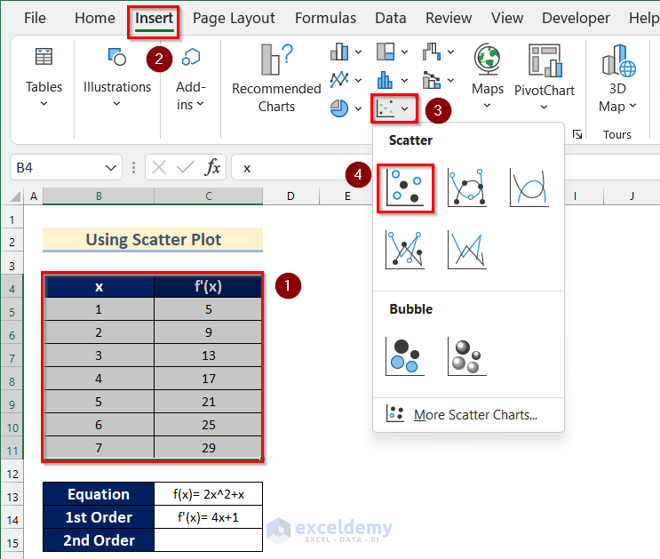
- A Scatter Plot will be inserted.
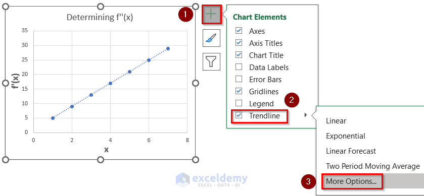
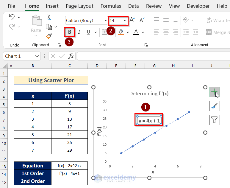
- Click on the “+” sign to open Chart Elements.
- Turn on Axis Titles.
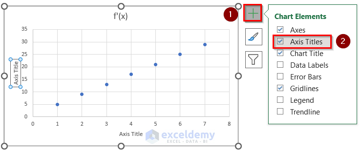
- Select the x-axis Title and type x.
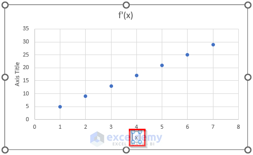
- Select the x.
- Select Font Size as 14 and click on Bold.
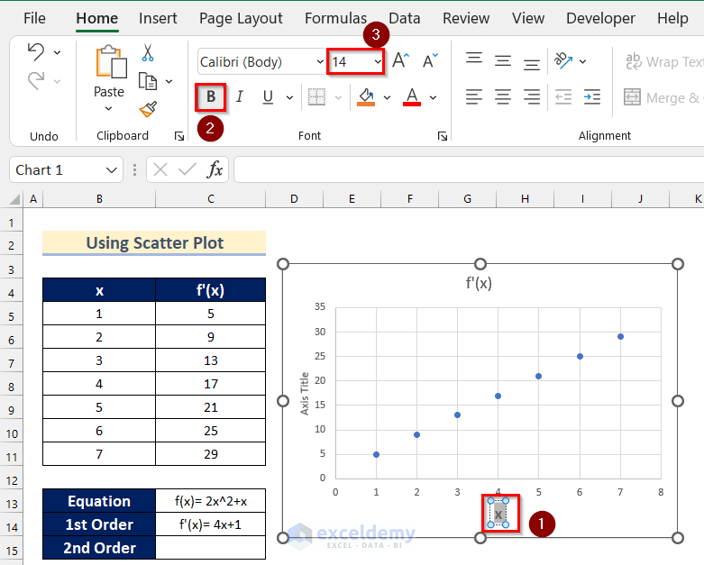
- Change the y-axis Title as f’(x) and format it.
- Select the Chart Title.
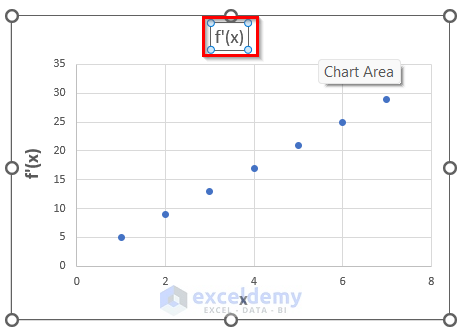
- Enter Determining f’’(x) as the Chart Title.
- Click on the “+” sign to open Chart Elements.
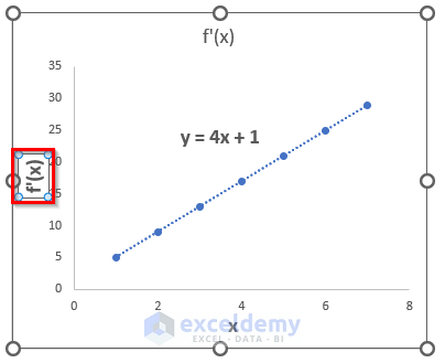
- Click on Trendline >> Select More Options.
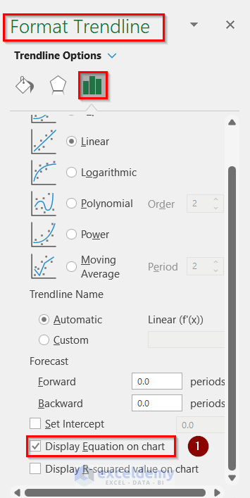
- The Format Trendline box will open.
- Select the Display Equation on chart option.
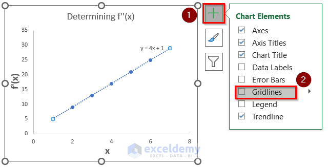
- Click on the “+” sign to open Chart Elements.
- Turn off Gridlines to see the equation.
- Select the equation.
- Set 14 as Font Size and click on Bold.
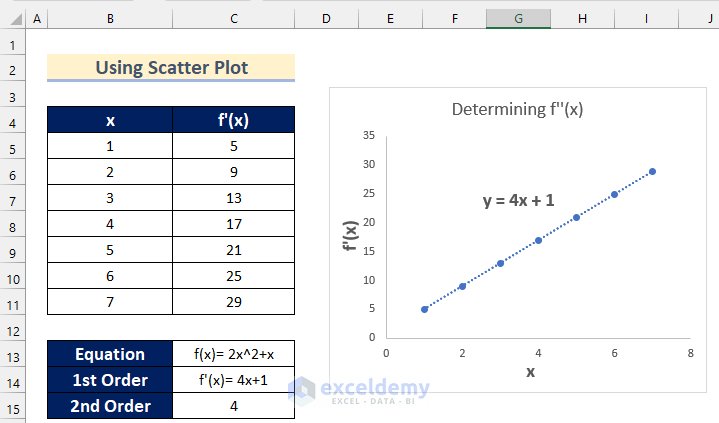
We get y= 4x+1 as the equation of the Trendline.
If we compare the equation with y= mx+c, we get m=4, the slope of the graph. We know that the slope of the 1st derivative and value of x of a function is equal to its second derivative. So, from the scatter plot, we get 4 as the second derivative of the function.
- Select cell C15.
- Enter the following formula:
=SLOPE(C5:C11,B5:B11)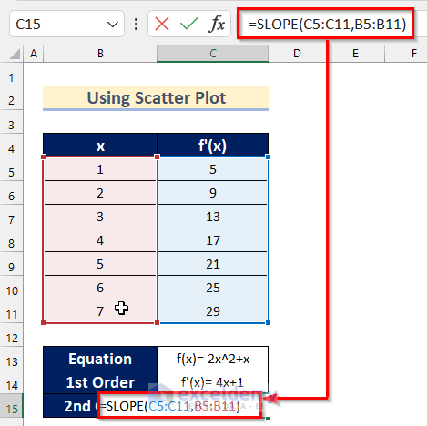
In the SLOPE Function, we used cell range C5:C11 as known_ys and Cell range B5:B11 as known_xs.
- Press ENTER.
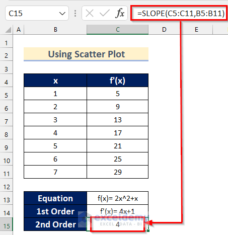
You will get the value of the Slope using the SLOPE Function.
You can see that the slope value is 4. So, the value of the second derivative of this function is 4.
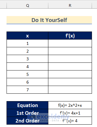
Practice Section
Here is the dataset to practice on your own and learn to use these methods.
Download the Practice Workbook
<< Go Back to | Calculus in Excel | Excel for Math | Learn Excel
Get FREE Advanced Excel Exercises with Solutions!
