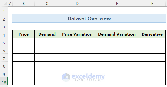
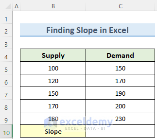
We’ll consider a simple dataset that contains the Price and the Demand columns. The Price will be in Dollars and the Demand will be in the number of units.
Step 1 – Inserting Input Data
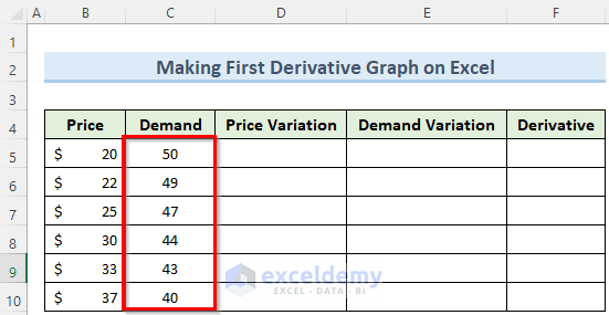
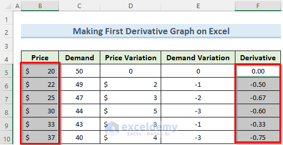
- Insert the Price data as in the image below in cells B5 to B10.
- Format the cells in column B as Accounting.

- Insert the Demand data in cells C5 to C10.
Step 2 – Creating Variations Columns
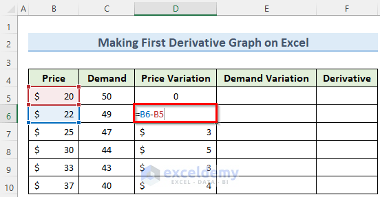
- Go to cell D5 and type 0.
- Use in the following formula in cell D6:
=B6-B5- Press the Enter key and copy the formula to the cells below. This will provide the Price Variation.
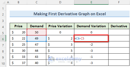
- Insert the following formula in cell E6:
=C6-C5- Press Enter and copy this formula to the other cells in the column.
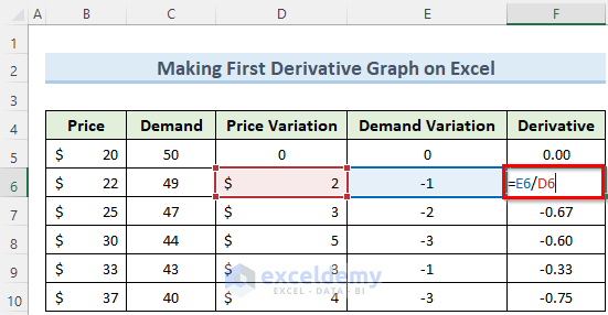
Step 3 – Finding the First Derivative
- Type 0 in cell F5.
- Insert the following formula in cell F6:
=E6/D6- Press Enter and copy this formula to the cells below using the Fill Handle.
Step 4 – Generating the First Derivative Graph
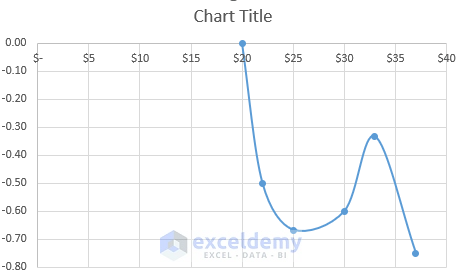
We will use a Scatter plot to clearly visualize the curve.
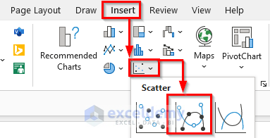
- Select the cells from B5 to B10 and F5 to F10 while holding the Ctrl key.
- Go to the Insert tab and, from the Scatter drop-down, select Scatter with Smooth Lines and Markers.
- This will generate the derivative graph reflecting the change in Demand with respect to Price.
Derivative Function in Excel to Find Slope
The SLOPE function in Excel returns the slope of a regression line based on some y and x values. This slope is actually the measure of the steepness of the data variation. In Mathematics, we use the formula as rise over run which is the change in y values divided by the change in x values.
Steps:
- Navigate to cell C10 and insert the following formula:
=SLOPE(C5:C9,B5:B9)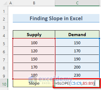
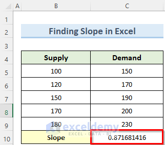
- Press the Enter key and you will get the slope for the input data.
Things to Remember
- If there is only one set of points, the SLOPE function will return #DIV/0!
- If the number of y and x values are not equal, the formula will return #N/A.
- To copy a formula to other cells, you can double-click on the Fill Handle instead of dragging.
Download the Practice Workbook
<< Go Back to | Calculus in Excel | Excel for Math | Learn Excel
Get FREE Advanced Excel Exercises with Solutions!
