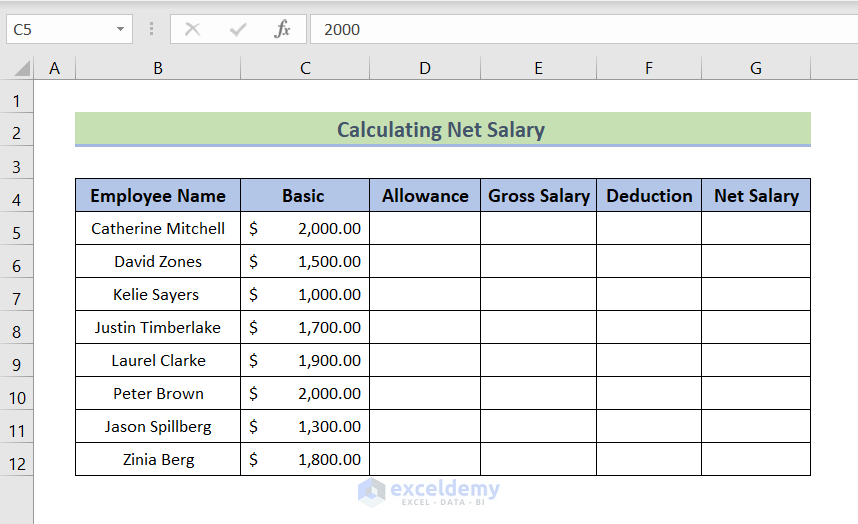
Method 1: Employee Database & Basic Salary Structure
The figure below shows basic salary structure of a company, and we want to calculate the net salary by adding allowances and subtracting deductions.
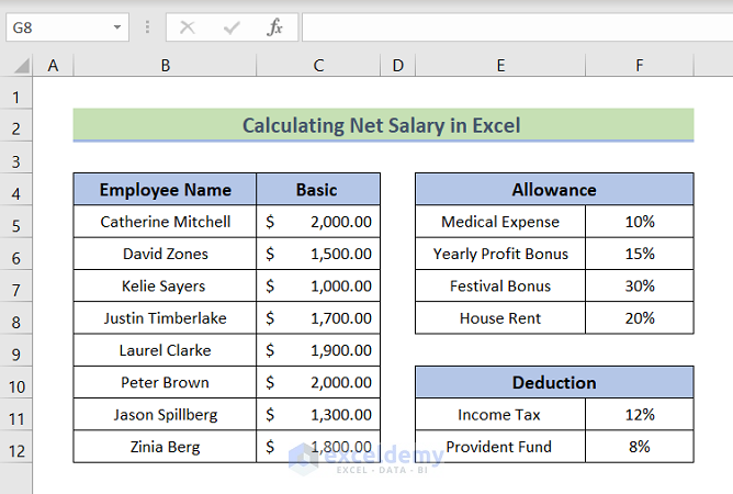
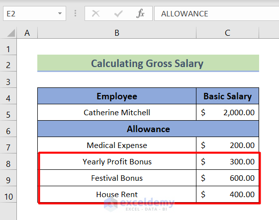
Method 2 – Create Allowance and Deduction Structure
The figure shows the allowance percentages of basic salary given by the company, among which medical expenses, yearly profit bonus, festival bonus, and house rent are included, and the deduction percentage of basic salary made due to provident fund and income tax.
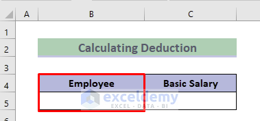
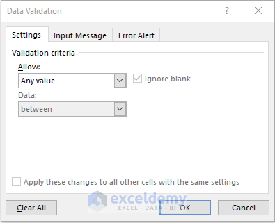
Method 3 – Apply Data Validation Feature
- Select cell B5.
- Use the Data Validation feature in this cell.
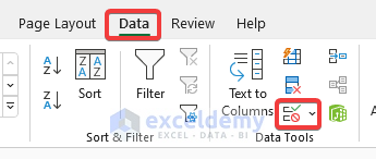
- Go to the Data Tab.
- From the Data Tools section, we select the Data Validation option.
- Select the Data Validation option, the Data Validation window will instantly pop up.
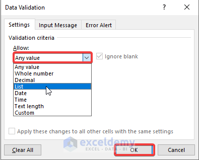
- From The feature Allow in the Data Validation window, we select List.
- Then OK.
- Insert the dataset range in the Source option.
- The range of datasets is:
=DATASET!$B$5:$B$12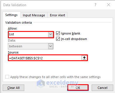
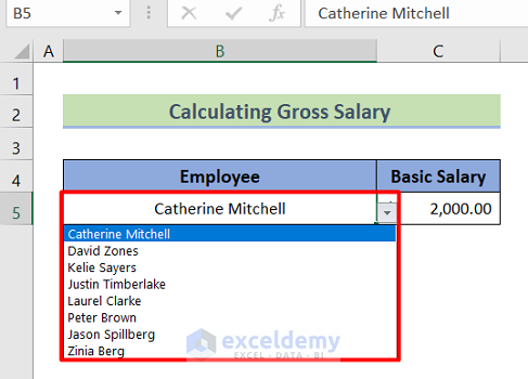
Method 4 – Calculating Gross Salary in Excel
- Gross Salary is the summation of basic salary and allowance.
- Use the Data Validation feature.
- A specific employee can be chosen from the list.
- Calculate the salary of Catherine Mitchell.
- Select the Dataset range.
- Use the VLOOKUP function of Excel.
- Use the formula in cell C5:
=VLOOKUP(B5,DATASET!B5:C12,2,FALSE)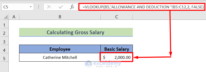
- Get medical expenses using the VLOOKUP function in cell C7.
- Get the Basic Salary of ‘Catherine Mitchell’.
- Get the medical expense the below formula is used:
=$C$5*VLOOKUP(B7,'ALLOWANCE AND DEDUCTION'!$E5:$F8,2,FALSE)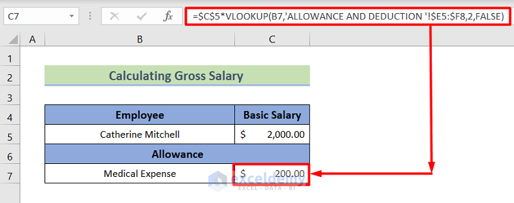
- VLOOKUP(B5,DATASET!B5:C12,2,FALSE)
The function searches for value cell B6 cell according to the Database values of employees in worksheets ranging from B5 to C12. It returns the respective 2nd column result from the following selection where the B6 cell’s value is found.
- $C$5*VLOOKUP(B7,’ALLOWANCE AND DEDUCTION ‘!$E5:$F8,2,FALSE)
$C$6 value is then multiplied by the result. The result is $200.00
- The total value of allowances can be calculated using the SUM function:
=SUM(C7:C10)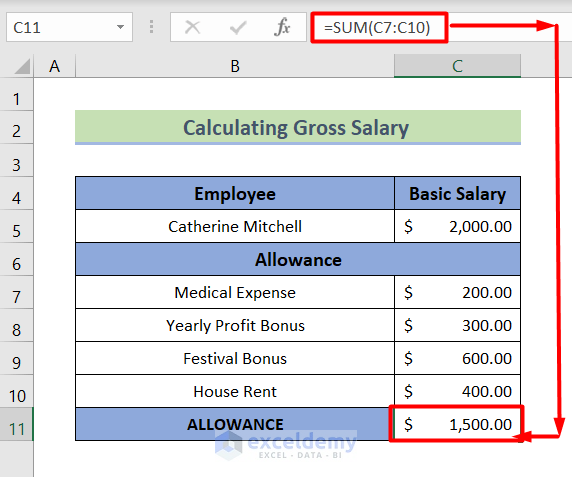
- Get the Gross Salary we use the SUM function in cell C6 and cell C14.
- Total Allowances through the below formula:
=SUM(C5, C11)- The result will look like the below image:
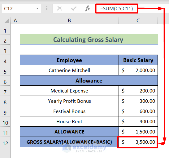
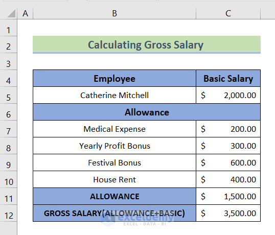
- Final outcome of the Gross Salary Calculation will look like the below image:
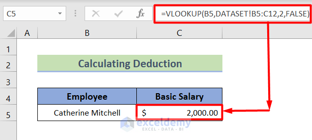
Method 5 – Deduction Calculation
- Use the Data Validation feature in cell B5.
- Calculate the Basic Salary using the formula below:
=VLOOKUP(B5,DATASET!B5:C12,2,FALSE)- The result will look like this:
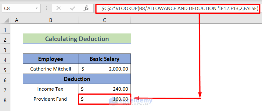
- Select cell C8.
- Calculate the income tax using the below VLOOKUP function formula:
=$C$5*VLOOKUP(B7,'ALLOWANCE AND DEDUCTION'!$E11:$E12,2,FALSE)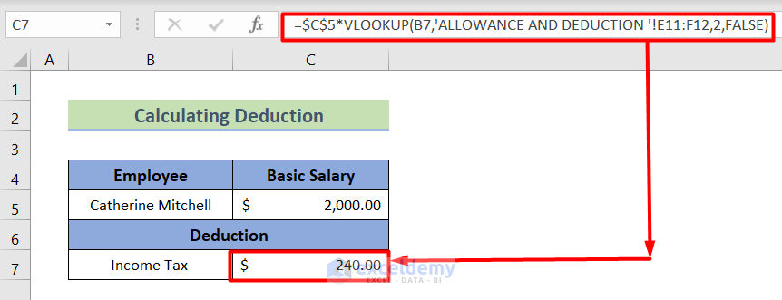
- VLOOKUP(B8,’ALLOWANCE AND DEDUCTION ‘!$E11:$E12,2,FALSE)
The VLOOKUP function searches for value cell B8 in the range E11:E12. It returns the respective 2nd column result from the following selection where we found the B8 cell’s value.
- $C$6*VLOOKUP(B8,’ALLOWANCE AND DEDUCTION ‘!$E5:$F8,2,FALSE)
The $C$6 value is then multiplied by the result. The result is $240.00.
- Use the Fill Handle tool.
- Get the provident fund amount as well.
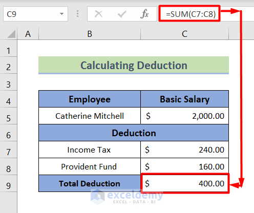
- At last, we use the SUM function in cell C11 to get the total deduction:
=SUM(C7:C8)- The final result will look like the below image:
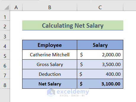
Method 6 – Calculating Net Salary
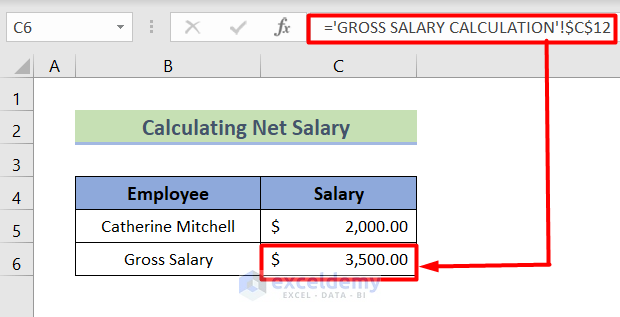
- Calculate Net Salary.
- Copy and paste the link to the Gross Salary in the Net Salary sheet.
- Use the below formula:
='GROSS SALARY CALCULATION'!$C$12- The result will look like the below image:
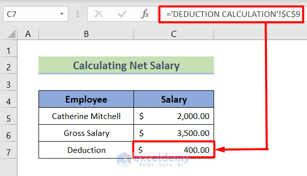
- Copy and paste the link into the net salary sheet.
- Use the below formula:
='DEDUCTION CALCULATION'!$C$9- The outcome will look like the below image:
- Select cell C8 and use the below formula:
=C6-C7- The final outcome will look like the below image:
Download Practice Workbook
Download the following workbook to practice by yourself.
<< Go Back to Salary | Formula List | Learn Excel
Get FREE Advanced Excel Exercises with Solutions!

You guys are doing such a wonderful job. I have been visiting your website for 3 days, to learn Excel formulas, and in a very short time, I have gained good knowledge of formulas. Keep doing good work team.
Hello Puri Nabaraj,
Thank you so much for your kind words! We’re glad to hear that our resources and blogs have helped you learn Excel formulas in such a short time. Your support motivates us to keep providing valuable content. Keep up the great work, and feel free to reach out if you have any questions or need further assistance!
Thanks again for your valuable feedback. Keep learning Excel with ExcelDemy!
Regards
ExcelDemy