Latest Posts From Nazmul Hossain Shovon

Method 1 - Typing Value in VBA to Add Text to Textbox in Excel Go to the Insert tab and click on the Text Box under Text. Click on the cell where ...

The dataset showcases Employee Name, Location (TextBox), and Location (Cell). Step 1 - Creating a Dataset Insert a column with the Employee ...
In the sample dataset, cells with monetary values are in Accounting format. Step 1 - Creating a Dataset Enter the Employee names in the first column. ...

In this tutorial, I am going to show you 2 simple methods to convert abbreviations to words in Excel. You can quickly use these methods even in large datasets ...
![[Fixed!] Excel Margins Disappeared (4 Possible Solutions)](https://www.exceldemy.com/wp-content/uploads/2022/11/excel-margins-disappeared-2.png?v=1697440073)
In this tutorial, I am going to show you 4 possible solutions to the Excel margins disappeared problem. You can quickly use these fixes even in large datasets ...

In this tutorial, I am going to show you 5 possible solutions to the Excel decimal places problem. You can quickly use these fixes even in large datasets to ...

In this tutorial, I am going to show you the step-by-step procedures on how to create a treemap with multiple levels in Excel. You can use these steps for any ...

In this tutorial, I am going to show you 3 ideal examples of how to use the paste name dialog box in excel. You can use these examples in your own dataset to ...
Dataset Overview Let’s assume we have a concise dataset with approximately 7 rows and 2 columns. Initially, all cells are in the General format, and monetary ...

In this tutorial, I am going to show you 3 simple methods on how to link Excel data to a PowerPoint chart. You can use these methods mainly in large datasets ...

In this tutorial, I am going to share with you 2 effective ways to create a real-time currency converter in Excel. You can easily apply these methods to ...
![[Fixed!] Excel Filter Stops at Blank Row (4 Possible Solutions)](https://www.exceldemy.com/wp-content/uploads/2022/11/excel-filter-stops-at-blank-row-5.png?v=1697441925)
We applied a filter to a dataset that has a blank row, but it stopped filtering when it encountered the blank row. Fix 1 - Selecting the Whole Range ...

Keep all the cells in General format. For all the datasets, we have 2 unique columns which are Items and Sales (units). We may vary the number of columns later ...

In this tutorial, I am going to show you 6 differences between Excel and Google Sheets formulas. From this, you will know when to use Google Sheets instead of ...

Method 1 – Using a Fill Handle Steps: Go to the lower-right corner of cell C5 and drag the + symbol down using the mouse. Click on the Auto Fill ...
- « Previous Page
- 1
- 2
- 3
- 4
- …
- 6
- Next Page »
See Our Reviews at


Hi Shruti,
I have attached an Excel file that you can use to find specific absent dates. Hope it helps!
Download link
Hi Maikel,
Can you share your Excel file with us, kindly? So that we may have a look at it and give you some suggestions.
Hi Cory,
You can follow the steps below for this:
1. Fill up the information in the pdf file. Then go to File >> Save as Text. This will create a file in .txt format.
2. Now open an Excel sheet. Go to the Data tab. Here in the top left corner, click on From Text/CSV and select the text file you just saved.
3. Finally in the next window, click on Load and this should bring the filled-in information as well.
Hope this helps!
Hi Mike,
You can try the following steps to change the date format in excel comments:
1) Type intl.cpl in the Windows Search Box.
2) Now, under Date and time formats, click on the Short date drop-down and choose the date format that you want to use in the comments in excel.
Hi James,
Thanks for your correction. To add, you can also calculate the GST amount using this formula:
GST Amount =
(C4*C5)/(1+C5)Then we can deduct this value of cell C6 from C4 to get the original price in cell C7.
Hi Brijesh,
I have created a simplified solution below. Please follow them:
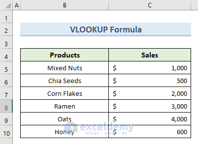
1. I am assuming that you have a Sheet1 like below:
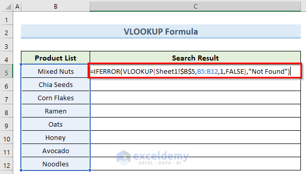
2. Now, go to the Sheet2 and insert the following formula in cell C5:
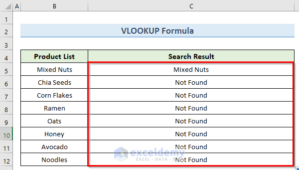
=IFERROR(VLOOKUP(Sheet1!$B$5,B5:B12,1,FALSE),"Not Found")3. Now, simply copy this formula down using Fill Handle and this should tell you whether the product in cell B5 inside Sheet1 exists in the Product List column or not.
Hi KARLHEINZ,
Looks like you have missed the <> symbol in the SMALL(IF((LEN($H$6:$H$13)0) portion of the formula. The correct formula should be this:
SMALL(IF((LEN($H$6:$H$13)<>0)
I hope this solves your problem. Please let us know if you face any other issues.