Latest Posts From Meraz Al Nahian

In this article, we will create a hierarchy tree of the following organization using different techniques. Method 1 - Using SmartArt Tool Steps: ...

Method 1 - Refreshing Google Sheets Step: Find that the formula is not working in Google Sheets, click on the Refresh button of the Sheets This ...
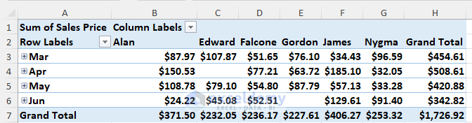
In this sample dataset there is sales data for a few products and the vendors that sold them in the months of March, April, May, and June. To convert ...

The COUNTF function counts data based on a single criterion. But when multiple ranges and matching criteria are involved, we can use its alternative, the ...
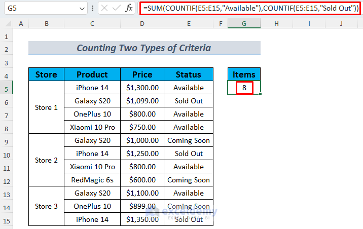
In this article, we’ll explore how to use the SUM and COUNTIF (or COUNTIFS) functions when dealing with multiple criteria in Excel.: The COUNT function is ...

The article will show you how to translate Portuguese to English in Excel. There may be a lot of ways to translate any language to English, but if you use ...
Here is a dataset that we will copy from Excel to Google Sheets. Method 1 - Enable Google Drive Offline to Copy Paste into Google Sheets ...
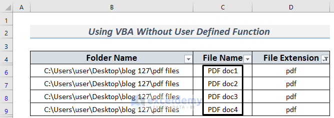
We can copy the names of the PDF files in a folder in various ways. A general presentation of an Excel sheet with PDF file names looks like the picture below. ...
The dataset below contains people’s Names, Mobile numbers, and Email addresses. We will use this data to create vCard files. Method 1 – Using ...

The article will show you how to calculate Confidence Interval without standard deviation in Excel. Basically, it’s easy to determine the Confidence Interval ...

In the dataset, you will see the profit data of a company for 4 years. The last one is the target profit (profit data in 2021). To achieve this, we will ...
Example 1 - Year-over-Year Comparison with a Bar Chart We have the data for goals scored by famous footballers in the 2016/17 and 2015/16 seasons. Let's ...
Method 1 - Using Excel Options Feature to Clear Recent Documents Steps: Go to the File tab. Click on Options. In the Excel Options ...
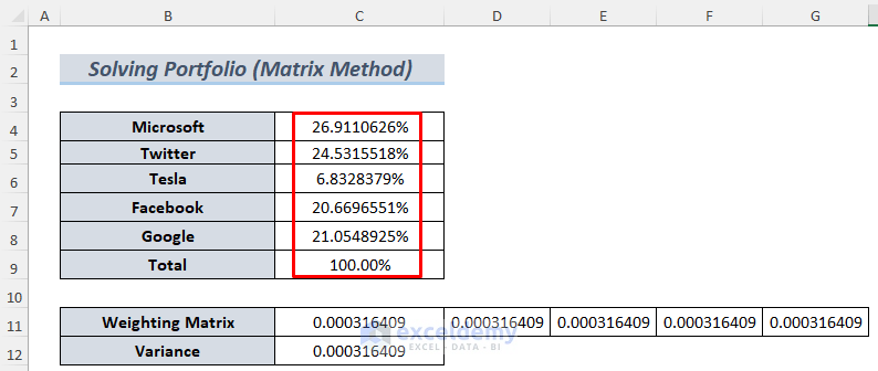
Method 1 - Using Matrix to Create Minimum Variance Portfolio (Multi Assets) Steps: Need to calculate the Excess Returns of these companies. Go to a new ...

The following picture shows an approximate model of a salary structure, which is based on employees’ experience. We will use the Regression Analysis tool to ...
- « Previous Page
- 1
- 2
- 3
- 4
- …
- 10
- Next Page »
See Our Reviews at


Hi VBANEWB, thanks for reaching out. Here, we declared Count variable first. So the VBA automatically accepts Count2 as a similar variable. So we didn’t need to declare it separately.
Hi Bates, Thanks for reaching out. Could you please share your dataset? That way, I might find the solution to your problem. Because, rows and columns both represent 2 dimensional array. It’s not generally possible to convert them to a 3d array.
Hi, Mr. Marais, thanks for reaching out. The way I see it, your time starts when you start travelling to your workplace and the end time is when your work time is over. So, subtracting 8 and half hour from this period of time (end time – travel start time) will provide the overtime. Also, Sundays and Holidays will be double overtime. Using this idea, I developed the following formula:
=IF(OR(B3="Sunday",C3="Yes"),2*((E3-D3)-TIME(8,30,0)),(E3-D3)-TIME(8,30,0))The image below is here for better clarification.
Hello Kellyn, thank you for reaching out. Here is a solution to your query. Use the code and replace the texts introduced by the OldLink and NewLink variables according to your preference.
Hi, Tan Li Wen, thanks for reaching out. Here, I developed a solution to your problem. I made a second column for email body in column B as shown in the picture.
Here is the modified code. Use it following the steps described in the previous comment.
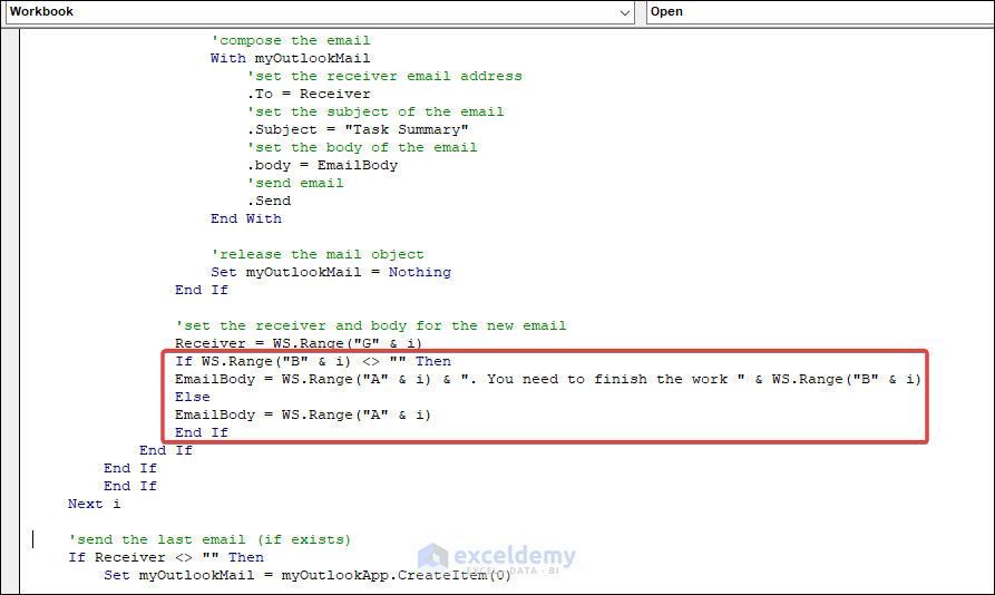
Here, I made changes in the marked portion of the following image. If there is a second message in the column B, it will be added to the main Email body as You need finish the work within ‘x’ days. If there’s no such thing in column B, only the part of the Email body in column A will be sent.
Hope this helps. If you have any more questions, please let us know in the comment sections.
Regards,
Md. Meraz Al Nahian
Team ExcelDemy
Hi Mr. Woods, thanks for reaching out. Here’s a quick solution to your problem. Just convert your data range to a table. If you enlarge the data range after that, the formulas will update accordingly and you will get your desired result.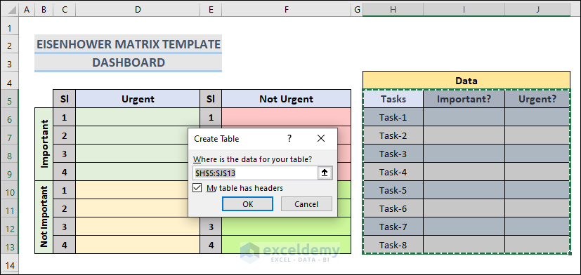
 However, here we made 4 4×1 matrices for different type of works. If you want to insert more tasks, just increase the rows corresponding important and not important tasks. I suggest you to go through the other comments if you haven’t already as you may find them useful.
I’m going to show the solution with images so you can understand this topic easily. First, I’m converting the Data range to a table. Select the marked range and press Ctrl + T to convert this range to a table.
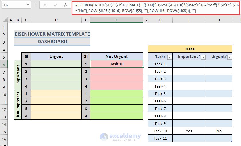
Now, add some rows to the table and insert the type of a task in the additional data range. You will see the task appear in the corresponding cell. Also, notice that the range in the formula updates automatically.
Hi Mr. Brown, thanks for reaching out. Regarding the solution of your problem, you just have to modify the code a bit. You can use the code of the 3rd method, but I don’t know why it takes 15 minutes to send the email to the receiver.
So, I used the code of the first method. I’m giving it here again with modification. See the image below to see where the modification is made.
You wanted to send the Email if the deadline is past 4 days by the current date. So I subtracted 4 in the code.
Remember, your desired date has to be present in the date list. I’m going to give you an example here. In the date list, the date 10/22/2023 is present. It is past 4 days by today’s date which is 10/26/2023.
If the date is not present in the list, the code will work but it won’t send any email. If you have any confusion, follow method 1 to operate the macro. You can insert necessary Email addresses and the message easily. Hope this helps you. Thank you.
Hello Rusty, thanks for reaching out. Your idea is correct. We don’t need to use the count2 variable here. Maybe it’s inserted to maintain the similarity with the previous line as it worked properly. Here is the updated code without the count2 variable. Hope this removes the confusion.
Hi, thanks for reaching out. Yes, there is a way to send emails with attachments using VBA. Here is the code for you.
You just have to change the file location according to your perception and use some valid email addresses. Also, keep logged into your outlook account.
Hi Mr. Pizzi, thanks for reaching out. I understand your confusion and you are correct. Our goal is to find out the maximum profit by varying the price. We will get the optimum amount of production that will provide maximum profit. As there is a fixed cost, the profit is dependent on the price. To find out the total profit, we have to multiply the quantity by the profit. Thanks again for your feedback.
Hi Jason, thanks for reaching out. I’ve used your formula and it returns PO for some values. However, I think I have a better idea for your solution.
Here, I made a drop down list using the names of the dataset (C5:C13 range). My target is, whenever you select a name, Excel will highlight the cell where the name last appeared.
Here is the drop down list.
And here is the formula with XLOOKUP and ROW functions to determine the row of last appearance of the name selected from the drop down list.
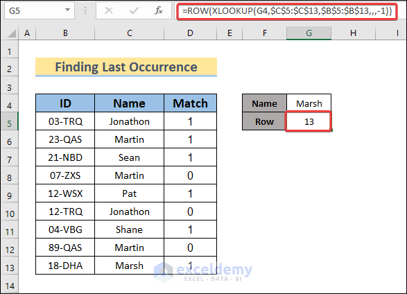
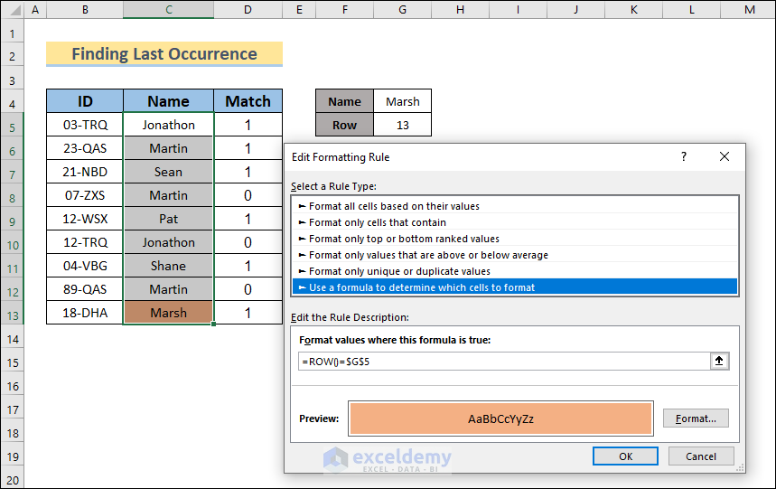
=ROW(XLOOKUP(G4,$C$5:$C$13,$B$5:$B$13,,,-1))To highlight the cell with the last occurrence, we need to set a formula for conditional formatting. So select the range of names (C5:C13) and then go to Home >> Conditional Formatting >> New Rule >> Use a formula to determine which cells to format and insert the formula below.
 Click the image to get a detailed view.[/caption]
=ROW()=$G$5[caption id="attachment_427897" align="aligncenter" width="750"]
After that, choose a fill color to format the cell and click OK.
Finally, if you select any name from the drop down, you will see the cell highlighted where the name occurred for the last time in column C.
Here, we selected Martin from the drop down and you can see that the name Martin appears 3 times in column C. But only the C12 cell is highlighted as it is the last time the name Martin appeared.
Hi Abhishek, thanks for reaching out! I also faced the same problem. The reason for this problem is that the API expires after a few days. You need to either update the API or create a new one. Then replace the old API in your Excel file with the new one. Hope this solves your problem.
Hello AC, thanks for reaching out. Here’s a solution to your problem.
Here, I have some addresses in two sheets. The addresses in the first sheet are in the left side of the following image. The addresses of the second sheet can be found in the drop down list.
And here is the formula to calculate the distance.
=ACOS(SIN(RADIANS(VLOOKUP(F3,Sheet2!A2:C33,2,FALSE))) *SIN(RADIANS(VLOOKUP(E3,A2:C29,2,FALSE))) +COS(RADIANS(VLOOKUP(F3,Sheet2!A2:C33,2,FALSE))) *COS(RADIANS(VLOOKUP(E3,A2:C29,2,FALSE))) *COS(RADIANS(VLOOKUP(F3,Sheet2!A2:C33,3,FALSE)-VLOOKUP(E3,A2:C29,3,FALSE)))) *6371Hi Andrija, thanks for reaching out. Actually there’s nothing wrong in the code. In my laptop, the code works properly. However, it may not work on other device. So I modified the code and updated the Download File in this article. I hope using the updated code will solve your problem.
Thanks David for your feedback. The formatting of Mix PY, Mix CY and Mix Change being in percentage made it a bit confusing. We’ll update it soon.
Hello Justin, thanks for reaching out. Here, the main formula for Mix Variance is:
Mix Variance = Revenue PY*(Price PY – Average Price PY)*(% of Mix CY – % of Mix PY). Although the Mix PY and CY were shown in percentage format in the article, we didn’t calculate these values as percentage. So in the formula, the difference of Mix CY and PY is divided by 100.
Hello JC, thanks for reaching out. Here, the main formula for Mix Variance is:
Mix Variance = Revenue PY*(Price PY – Average Price PY)*(% of Mix CY – % of Mix PY). Although the Mix PY and CY were shown in percentage format in the article, we didn’t calculate these values as percentage. So in the formula, the difference of Mix CY and PY is divided by 100.
I hope you need something like this- once you update the status of a work in a column, there will be a strikethrough in the Eisenhower dashboard.
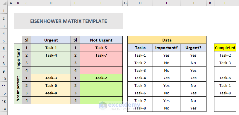
Here is a sample how you can work with it.
You can see that the completed tasks (Task-2, Task-3 etc.) get a strikethrough in the Urgent and Not Urgent columns. For this purpose, we will apply two conditional formatting for two types of work (Urgent and Not Urgent). Select the Urgent range first and then go to Conditional Formatting >> New Rule.
The New Formatting Rule window will appear. Select the option Use a formula to determine which cells to format and type the formula below in the ‘Format values where this formula is true‘ section.
[wpsm_box type="red" float="none" textalign="center"]
=OR(D6=$L$7:$L$14)[/wpsm_box]
After that, click on the Format button.
In the next window, check Strikethrough and click OK.
You will see a preview of how the formatted texts will look like, just click OK.
Finally you will see the Strikethroughs on the Completed Urgent tasks in the Eisenhower dashboard.
Do the same Conditional Formatting procedure for the Not Urgent range. You will get Strikethroughs on Not Urgent Completed tasks.
Please mention which method you are following, this will help us to understand the reason why this error is occurring. Thank you.
Hello Winsett, thanks for reaching out. In that case, use SUM function to calculate the total cost. Also, you can find the total cost automatically in the bottom right corner of your Excel sheet for the selected data. To sum the cost by criteria, use the SUMIF/SUMIFS function.
Hello Zeus, thanks for reaching out. If you want the sales data for Rowan and Ben in a single column, you simply insert the names Ben and Rowan in the new Name column (Cells B13 and B14). Putting the original formula in cell C13 will return the sales data about Rowan. Then you just drag the Fill icon downwards to copy the formula in C14 which will show the data of Ben. Putting names multiple times in the output part is not necessary. This will incident redundant result.
Hello Ahmed, thank you for reaching out. You can send email in a certain time of a day automatically, but you have to keep the Excel file open. One more thing, you cannot send email automatically by Excel everyday. You have to set up the time and then run the Macro. The code is given below.
In the picture, I’m providing you some direction regarding where you may need to change the code element.
Note: If the code doesn’t work, make sure you have an Outlook account and open the Microsoft Office App.
Thank you Julie for reaching out. The first method can be done to solve your problem. Just copy the data and paste this as linked picture into a new spreadsheet. Any change in your main spreadsheet will automatically be updated in the new sheet.
Hi Medha, Thanks for reaching out. Please try this code below. Hope this is the solution to your problem.
The message text in the second is actually the mail body. If you want to change the Subject of the email, you can simply change it in the code. Please follow the code in the picture below. This subject will be the same for all the mails.
Hey Barry, thank you for reaching out. If you provide your workbook, that would be easy for me to understand your problem.
Hello L.C., thank you for reaching out. The angles in the formula are used as input for the Sine and Cosine functions. So the conversion from degree to radian isn’t necessary. Whether I change the angle unit to radian or not, the value of the corresponding Sine or Cosine function will be the same as the angles remain the same.
Hey Pam, it’s really nice to see you get benefit from my article. It’s also an honor because I work with sincerity for these articles so the readers can have their solutions in the easiest way possible. I appreciate your compliment and also hope that my other articles can be useful for you as well. You are welcome!!!
Hello Melissa, thanks for reaching out. To answer your question, yes, you can export data from that PDF file to Excel. Just for a reminder, when you do that, please follow the steps.
1. Open the PDF file in Adobe Acrobat Pro.
2. Then select Tools >> Forms >> More Form Options >> Merge Data Files into Spreadsheets.
By doing this, you can export everything from your fillable PDF file to Excel Spreadsheet.
Hello Michael, thank you for reaching out. We will be working on this matter in MAC and update the article with this information. Right now, please try the code below. Hope this will be useful for you.
The code should save the document as PDF and the name of the document will be followed by the text in the B4 cell of your Excel sheet.
Hi Dav, thank you for reaching out. It’s unavoidable to have empty cells after the name of the players because we are splitting the adjacent cells to the Footballer Name column.
Hello Mr. Gurry, thank you so much for the feedback. I have updated the article according to your suggestions. What I did before is that I tried to use the xlOr operator for two different AutoFilter Field. But this can be done by With Statement and I showed the process in Method 1. Here I changed the conditions too. Please check again if there’s anything you want to add.
Hello sir, the process has been disabled since May 31. But to be sure, please check your Google account if you have the option ‘Less secure app access’ available. You can find this option from Manage Account >> Security >> Less secure app access. If you enable this option, then you can send Mails without Outlook.
Hi Msirhc, thanks for reaching out. This actually happens because you haven’t typed the proper column in the first input box that shows up after running the code. The rows are inserted based on values, so if you select the first column (The week column), it won’t work, because that column contains text, not values. The second and third column of the dataset contain values. But the sales column contains irrelevant large values. So you should type 2 in the first input box if you want to use this dataset.
Hey Praveen, thanks for reaching out. This XML files are actually in version 1 format.
Hi BZ, thanks for your response. You can reference the cells from one sheet to another workbook. That way, you can automatically update data in the new workbook when you make a change in the existing worksheet. And to update with condition, you need to use conditional function like the IF, AND, OR, EXACT etc. functions.
Hello Shan, thanks for reaching out. It would be good if you share your code and the dataset file so that I could understand your problem clearly. What I understand from your comment, I think it is not the problem. You need to get your hidden rows back after you delete the filtered data. And to do that, just press CTRL+SHIFT+L. The command will remove the filter and return your hidden rows back.
Hi Cavallino, thanks for reaching out. The good news is, you can send emails by VBA using Outlook. Please check this article “How to Automatically Send Emails Based on Date“. You can also find similar articles on our website. Hope this will help you.
Hi Dabrowski, thanks for reaching out. If you remove the ‘& LastRowFind(“convertxml”)’ part from the 7th line of the code. It will solve your problem. The function ‘LastRowFind’ causes to generate that extra file.
Hey Bharat, thanks for reaching out. Could you specify the code that face problem using it?
That’s great Griffin, I hope you get benefited from our articles.
Hi Tanya, thanks for reaching out. I understand your problem. It may not be possible to send the Email just by running the code and wait for the day to come. But I can help you on sending email at a certain time in a day. The 3rd code sends email in the current date when you run it. You can add a scheduler in the code. The email will be sent at the time you set in the code. I added the code below. You can see that the time here is 16:18:00. So if you run the code before 16:18, and keep the corresponding Excel file open, the email will be sent at 16:18. You don’t need to rerun this code during this time. Hope this helps you a bit. I’ll be working on your problem too. If I get a solution, I’ll immediately add that in your reply.
Option Explicit
Private Sub Workbook_Open()
Application.OnTime TimeValue(“16:18:00”), “SendEmail03”
End Sub
Sub SendEmail03()
Dim Date_Range As Range
Dim rng As Range
Set Date_Range = Range(“B5:B10”)
For Each rng In Date_Range
If rng.Value = Date Then
Dim Subject, Send_From, Send_To, _
Cc, Bcc, Body As String
Dim Email_Obj, Single_Mail As Variant
Subject = “Hello there!”
Send_From = “[email protected]”
Send_To = “[email protected]”
Cc = “[email protected]”
Bcc = “”
Body = “Hope you are enjoying the article”
On Error GoTo debugs
Set Email_Obj = CreateObject(“Outlook.Application”)
Set Single_Mail = Email_Obj.CreateItem(0)
With Single_Mail
.Subject = Subject
.to = Send_To
.Cc = Cc
.Bcc = Bcc
.Body = Body
.Send
End With
End If
Next
Exit Sub
debugs:
If Err.Description <> “” Then MsgBox Err.Description
End Sub
Hi Bolton, thanks for reaching out. I think you need to use different code for your solution. The following code will create a user defined function to sum up the data based on the background color of cells.
Function SumBasedOnColor(mn_cell_color As Range, mn_range As Range)
Dim mn_sum As Long
Dim mn_colorIndex As Integer
mn_colorIndex = mn_cell_color.Interior.ColorIndex
For Each mn_CI In mn_range
If mn_CI.Interior.ColorIndex = mn_colorIndex Then
mn_sum = WorksheetFunction.Sum(mn_CI, mn_sum)
End If
Next mn_CI
SumBasedOnColor = mn_sum
End Function
After that, use the function like the following image.
There’s something important that you have to keep in mind. We referenced the cell F4 here and this cell background color was filled with yellow. The cell you reference should have the background color matched with the cells containing data.
Hi Samad, thank you for reaching out. Fortunately there is a way to automate sheet name based on a cell value. In the image, you can see that I have a cell value in A1. I also have values in A1 cell of the other sheets. I will change the name of the corresponding sheets based on the value in A1.
Now, type the following code in a VBA module and run it.
You can see that the name of the sheet changes according to the cell value of A1. If you store sheet names in another cell such as B5, you need put this cell reference instead of A1 in the VBA code. Otherwise you will encounter errors.
Hi Steve, we are extremely sorry for your trouble. Named ranges are pretty useful when we need to use a range repeatedly. A lot of our readers are okay with it. Going through the dataset can help anyone to understand the defined range of a named range. But we are taking your feedback sincerely. We’ll apply your suggestion in the upcoming articles.
Hi Kinney, thanks for your response. The formula was actually written in cell E6. It was a typing mistake in the description of the process. We are extremely sorry for you to have trouble on this matter.
Hi Shilpa, thanks for the response. Here’s the solution to your question no 1
You can simply create a criteria similar to the methods of this article using dates. Suppose you want to see the sales information after May. Please watch the following image for the process. I created the criteria in G6 cell.
In order to solve the second question of your comment, please apply the method described in the Section 3.2 of this article.
Hope this helps to solve your queries.
Hi Mary, thanks for your response. You can definitely apply this process in a single sheet. However we use different sheets to show the different processes for the same output. And it also seemed convenient to use separate sheets to show the application of using the data validation list for different conditions. So different sheets for different methods were used in this article. Hope that provides you with the answer to your question.
Hello sir, thank you for the feedback. We are working hard on this matter, I hope we will provide you the solution in the upcoming tutorial pretty soon.
Hi Pranav, thanks for the query. You can simply use the code of the second method of the article in this regard. Just follow the procedure after you run the code. Hope that helps you.
Hi! Thanks for asking. As the article was to provide some templates, I didn’t go in detail with the formula. Here, Invoice_Info is a named range. It refers to the range B12:J17 of the ‘template 1’ sheet. To create a named range, you need to select your desired range of cells, then go to Data Tab >> Define Name and after that, give a name of that range. The advantage is that, you can use that range by inserting it’s name anywhere in the worksheet or workbook. You don’t have to select the range every time you use it in a formula. Hope this solves your problem.
Thank you Sir! I hope you will find my other articles useful and enjoyable too. Please visit this Link to explore more!
hi Chris, thanks for your response! A possible reason could be that you may not have the original or latest version of Adobe. If that’s the case, please install that. Hope this helps.
hi, thanks for asking Liss. It will be better for you to use the code of the second method. You may not be able to set a reminder using VBA, but you can set a date interval using it. If you go through the explanation, you will see that I created a 7 days interval in the code (you can change it according to your convenience). If you want to remind your employee that he should finish his job within a week, you can use the dataset and VBA code of the second method. You cannot send emails on a particular date. Suppose you run this code on 15th July. You have a date range of 15th July to 25th July. The employees who have to finish their task within 16th to 22nd July will get your mail. Those who have to finish within 23rd to 25th won’t get your mail. However, you can make a schedule to send your mail in a particular time of the day. Just put the following statement at the beginning of the code of the second method. Hope this helps
Option ExplicitPrivate Sub Workbook_Open()
Application.OnTime TimeValue("hh:mm:ss"), "SendEmail02" 'put the time when you want to send the email
End Sub 'you must keep open your excel file until then after you run the code
hello there, thanks for asking. I understand your problem. Although I haven’t found the exact solution to your problem yet, I can help you on sending email at a certain time in a day. The 3rd code sends email in the current date when you run it. You can add a scheduler in the code. The email will be sent at the time you set in the code. I added the code below. You can see that the time here is 16:18:00. So if you run the code before 16:18, and keep the corresponding Excel file open, the email will be sent at 16:18. You don’t need to rerun this code during this time. Hope this helps you a bit. I’ll be working on your problem too. If I get a solution, I’ll immediately add that in your reply.
Option Explicit

Private Sub Workbook_Open()

     Application.OnTime TimeValue("16:18:00"), "SendEmail03"

End Sub

Sub SendEmail03()

Dim Date_Range As Range

Dim rng As Range

Set Date_Range = Range("B5:B10")

For Each rng In Date_Range

If rng.Value = Date Then

Dim Subject, Send_From, Send_To, _

Cc, Bcc, Body As String

Dim Email_Obj, Single_Mail As Variant

Subject = "Hello there!"

Send_From = "[email protected]"

Send_To = "[email protected]"

Cc = "[email protected]"

Bcc = ""

Body = "Hope you are enjoying the article"

On Error GoTo debugs

Set Email_Obj = CreateObject("Outlook.Application")

Set Single_Mail = Email_Obj.CreateItem(0)

With Single_Mail

.Subject = Subject

.to = Send_To

.Cc = Cc

.Bcc = Bcc

.Body = Body

.Send

End With

End If

Next

Exit Sub

debugs:

If Err.Description <> "" Then MsgBox Err.Description

End Sub