Latest Posts From Mashhura Jahan

To demonstrate how to use Excel VBA to scrape data from a website using the Chrome browser, we'll use this article from ExcelDemy as the dataset, and scrape ...

We'll the following Excel sheet to showcase decryption. It contains a sales overview. If I try to edit something in this Excel sheet it shows a Warning ...

There are many ways of calculating Depreciation. Units of Production is one of them. The main objective of this article is to explain how to calculate the ...
What Is NPV? NPV, or Net Present Value, is a fundamental component of financial analysis. It helps determine whether a project will be profitable. The NPV ...

A data table helps to represent data more clearly in an Excel chart. If you are looking for a way of editing a data table in an chart then you have come to the ...
Example 1 - Sort Sunburst Chart Order Alphabetically in Excel Step 1 - Insert Sunburst Chart Select the data range for the chart. Go to the Insert tab ...
Codes for Different Languages Here's a short list of language codes for some languages. You will find the detailed list on the Google Cloud web link. ...
Dataset Overview Let’s take a closer look at our dataset. It includes two columns: “Date” and “Sales.” This data is visualized using a column chart. We’ll use ...

Dataset Overview We'll use the following dataset to explain these methods. It contains 3 columns, State, Product, and Sales. Method 1 - COUNTIFS ...

The COUNTIF function is one of the statistical functions. This function is used to count cells that meet a certain criterion. The focus of this article is to ...

This dataset contains 3 columns State, Department, and Sales Person. Let's show how you can translate this Excel file from English to Gujarati. ...

The VLOOKUP Function The VLOOKUP function looks for a given value in a data range and returns the exact match or an approximate match of that value. ...
This is the sample dataset. A filter was applied for Texas, but it is not working after row 6. Reason 1 - Blank Cells in the Range To ...
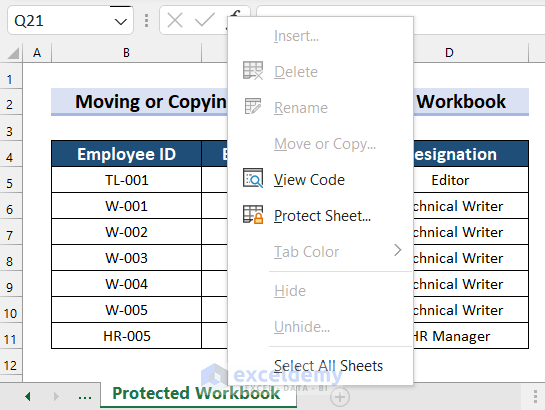
The below dataset contains employee Information: Employee ID, Name, and Designation. Reason 1: Having an Excel Table in Grouped Worksheets If you ...

If you are looking for a way to automatically convert your Excel file to Google Sheets then you have come to the right place. The objective of this article is ...
- « Previous Page
- 1
- 2
- 3
- 4
- …
- 7
- Next Page »
See Our Reviews at


Hi DOUG KIMZEY,
Thank you for your comment. I am replying on behalf of ExcelDemy. Power Query sometimes shows grayed-out menus if you try to perform mathematical operations in multiple columns at the same time.
• To solve that problem, you can select the column >> select Standard >> select Divide (or whatever operation you want).
• Select the Value according to your preference. Here, I want to divide by 200 because these scores are in 200 >> select OK.
• Now, you can see the values in the column are divided by 200.
• In the formula bar, add your preferred operations >> click on the Tick mark.
• Finally, you will see that you have performed the grayed-out features without using them.
If this tip doesn’t work for you then please share a screenshot of your problem or the Excel file with us so that we can see what is causing the problem and solve it.
Regards,
Mashhura Jahan
ExcelDemy.
Hi DANIEL,
Thanks for your comment. I am replying to you on behalf of ExcelDemy. You can apply the following formula to insert the first date in the ‘daily’ section to get the correct weekday name.
=TEXT(AM11,"DD")Use the following formula for the second date.
=TEXT(K4+1,"DD")Also, modify the rest of the dates accordingly to get the correct result. I hope this will help you to solve your problem. Please let us know if you have other queries.
Regards,
Mashhura Jahan
ExcelDemy.
Hi PIET,
Thanks for your comment. I am replying to you on behalf of ExcelDemy. You can apply the following code. By using this code, you will be able to double-click on any cell from columns C, G, or L and the entire range (A4:L60) will be sorted based on the column of the selected cell.
I hope this will help you to solve your problem. Please let us know if you have other queries.
Regards
Mashhura Jahan
ExcelDemy.
Hi OMAR DEL VALLE,
Thanks for your comment. I am replying to you on behalf of ExcelDemy. You can apply the following formula for finding duplicate barcodes.
=IF(COUNTIF($C$5:C5,C5)>1,"Duplicate",Code128(C5))But, here the duplicates are also in Code 128 font to change that follow these steps.
• Right-click on the sheet name >> select View Code.
• Write the following code.
• Now, just drag the Fill Handle and you will get your desired result.
I hope this will help you to solve your problem. Please let us know if you have other queries.
Regards
Mashhura Jahan
ExcelDemy.
Hi RICHARD O’CONNOR,
Thanks for your comment. I am replying to you on behalf of ExcelDemy. You can apply the following formula to calculate working days until a future date. And then, drag the fill handle down to copy the formula in other cells.
=NETWORKDAYS.INTL(C5,D5,1,$G$5:$G$9)Here, Cell C5 is start_date, D5 is end_date, 1 refers to Saturday and Sunday as the weekend, and range $G$5:$G$9 refers to the holidays.
Note: If you skip weekend and holidays arguments in the formula then it will take Saturday and Sunday as weekends and no holidays.
I hope this will help you to solve your problem. Please let us know if you have other queries.
Regards
Mashhura Jahan
ExcelDemy
Hi JHON,
Thanks for your comment. I am replying to you on behalf of ExcelDemy. If you insert pictures with text in the same cell like the following dataset, you will be able to search the pictures easily by following the first method from this article.
In the following image, you can see that the results for the router are displayed with pictures.
For this case, you will have to set the Properties for the pictures as Move and size with cells from the Format Graphic task pane.
I hope this will help you to solve your problem. Please let us know if you have other queries.
Regards
Mashhura Jahan
ExcelDemy.
Hey NICO,
Thank you for your comment. I am replying on behalf of ExcelDemy. You can use the IF function to check through every error group. The formula will be something like this:
ID=IFERROR(IF(error group = 1,TEXTJOIN(“, “,TRUE,FILTER(ID array ,error group 1 array=”x”,””)),IF(error group = 2,TEXTJOIN(“, “,TRUE,FILTER(ID array ,error group 2 array=”x”,””)),IF(error group = 10,TEXTJOIN(“, “,TRUE,FILTER(ID array ,error group 10 array=”x”,””)),””))) ,””)I hope this will help you to solve your problem. Please let us know if you have other queries.
Regards
Mashhura Jahan
ExcelDemy.
Hey EXC,
Thank you for your comment. I am replying on behalf of ExcelDemy. If you are facing this problem with Method 1 then you will have to select the reference cell in the formula from the first row of the range you are selecting. You can see that range C5:D12 is selected in this article. And, cells C5 and D5 were used in the formula. These cells are in the first row of the selected range. You will have to maintain this rule while writing the formula.
I hope this will help you to solve your problem. And, if it doesn’t, let us know in which method you are facing the problem.
Regards
Mashhura Jahan
ExcelDemy.
Hi BIANKA,
Thanks for your comment. I am replying to you on behalf of ExcelDemy. If you want to get the distance in KILOMETERS then you can use the following VBA code and the rest of the procedures will be the same.
I hope this will help you to solve your problem. Please let us know if you have other queries.
Regards
Mashhura Jahan
ExcelDemy.
Hello ZAIN,
Thanks for your comment. I am replying to you on behalf of ExcelDemy. For Example 5, you will have to keep 2 things in mind.
1. You will have to change the ColumnCount in the ListBox Properties according to your dataset.
2. In the VBA code, you will have to change Row and Column numbers according to your dataset.
I hope this will help you to solve your problem. If it fails to solve your problem, then please specify where are you facing the problem.
Regards
Mashhura,
ExcelDemy.
Hi XIONG YANG,
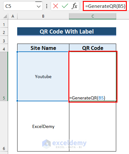
Thanks for your comment. I am replying on behalf of ExcelDemy. You can not add a label directly in the QR Code. But, you can add a label to the cell where you are inserting the QR Code by following these simple steps.
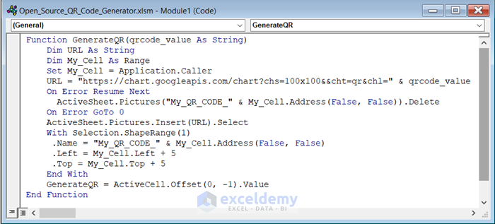
Step-01: Write the following VBA code in the module instead of the code that is provided in this article.
Function GenerateQR(qrcode_value As String)Dim URL As StringDim My_Cell As RangeSet My_Cell = Application.CallerURL = "https://chart.googleapis.com/chart?chs=100x100&&cht=qr&chl=" & qrcode_valueOn Error Resume NextActiveSheet.Pictures("My_QR_CODE_" & My_Cell.Address(False, False)).DeleteOn Error GoTo 0ActiveSheet.Pictures.Insert(URL).SelectWith Selection.ShapeRange(1).Name = "My_QR_CODE_" & My_Cell.Address(False, False).Left = My_Cell.Left + 5.Top = My_Cell.Top + 5End WithGenerateQR = ActiveCell.Offset(0, -1).ValueEnd FunctionNow, Save the code and go back to your worksheet.
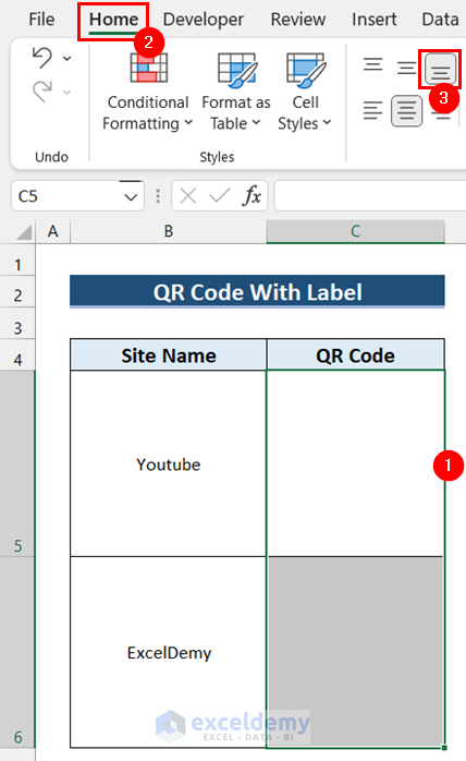
Step-02: Select the cells where you want the QR Codes >> go to the Home tab >> select Bottom Align.
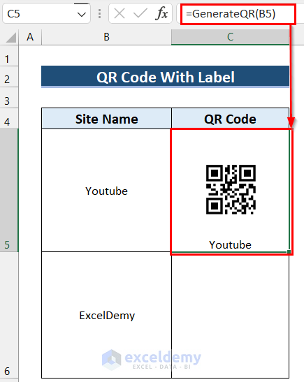
Step-03: Select the cell where you want the QR Code >> write the following formula in that cell.
=GenerateQR(B5)Next, press Enter and you will get the QR Code with the Label.
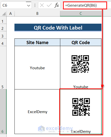
Step-04: Finally, get the QR Codes for other data in the same way.
I hope this will help you to solve your problem. Please let me know if you have other queries.
Regards
Mashhura,
ExcelDemy.
Hey ERIK NIELSEN,
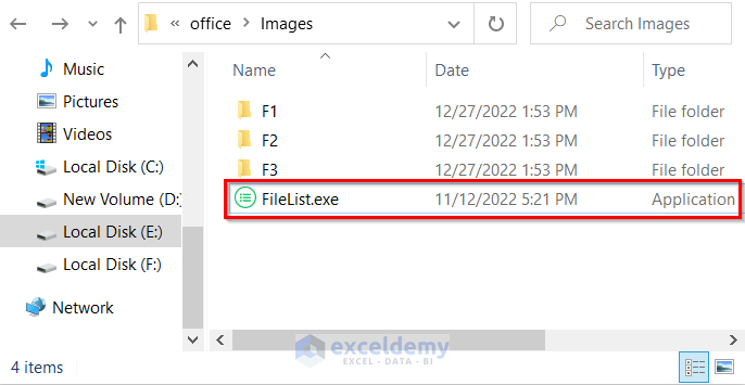
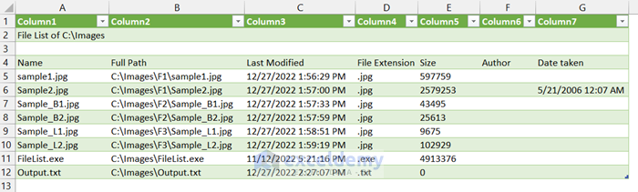
Thanks for your comment. I am replying to you on behalf of ExcelDemy. If you want to get metadata from subfolders of the specified source folder then you can use the jamsoftware that is used in the “How to Export File Metadata to Excel” section of this article. Let’s see the steps.
• Firstly, download and then copy and paste the FileList.exe file to the folder from where you want to get the metadata by following the steps from the “How to Export File Metadata to Excel” section of this article.
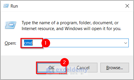
• Secondly, press Windows Key + R.
• Thirdly, write cmd in the Open section.
• Then, select OK.
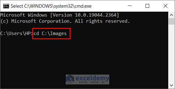
• After that, write
cd C:\Images. Here,C:\Imagesis the source folder path.• Then, press Enter.
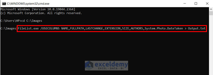
• Next, write the command below.
FileList.exe /USECOLUMNSNAME,FULLPATH,LASTCHANGE,EXTENSION,SIZE, AUTHORS,System.Photo.DateTaken > output.txt• Then, press Enter.
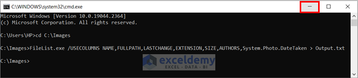
• After that, minimize the window.
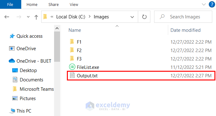
• Now, you will see a txt file is created in your selected location. It contains the metadata from all the subfolders.
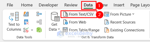
• Next, open an Excel file >> go to Data tab >> select From Text/CSV.
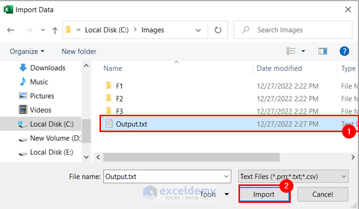
• Afterward, select the txt file >> select Import.
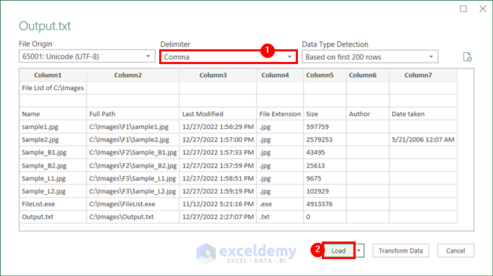
• Now, you will see the metadata are imported to a table.
• Then, select Comma as Delimiter >> select Load.
• Finally, you will see all the metadata from the subfolders is loaded to an Excel sheet.
I hope this will help you to solve your problem. Please let me know if you have other queries.
Regards
Mashhura,
ExcelDemy.
Hey MARK,
Thanks for your comment. I am replying to you on behalf of ExcelDemy. For the provided practice workbook, I used the following VBA code and it solved this problem for me.
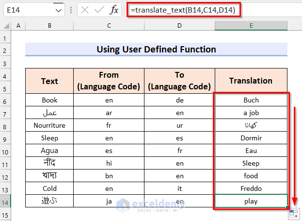
Function QR_Generator(qrcodes_values As String)Dim Site_URL As StringDim Cell_Values As RangeSet Cell_Values = Application.CallerSite_URL = "https://chart.googleapis.com/chart?chs=100x100&&cht=qr&chl=" & qrcodes_valuesOn Error Resume NextWorksheets("Using User Defined Function").Pictures("Generated_QR_CODES_" & Cell_Values.Address(False, False)).DeleteOn Error GoTo 0Worksheets("Using User Defined Function").Pictures.Insert(Site_URL).SelectWith Selection.ShapeRange(1).Name = "Generated_QR_CODES_" & Cell_Values.Address(False, False).Left = Cell_Values.Left + 2.Top = Cell_Values.Top + 2End WithQR_Generator = ""End FunctionNow, Save the code and go back to your worksheet. Let’s see the steps of using the function.
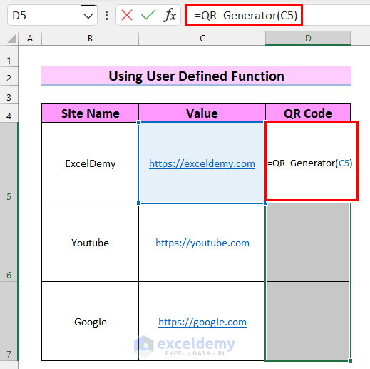
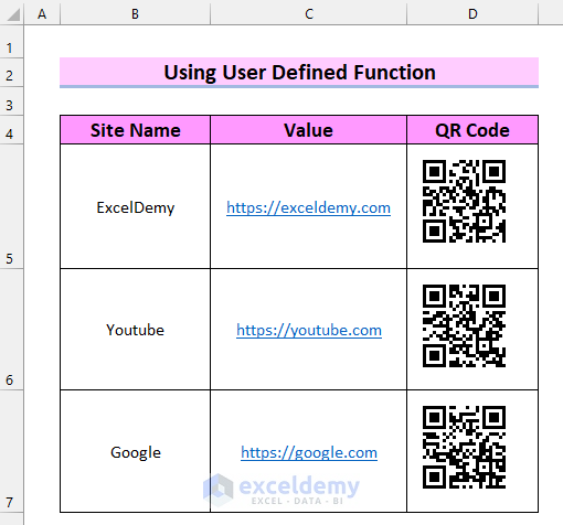
Step-01: Select the cells where you want the QR Codes. Here, I selected cell range D5:D7 >> write the following formula.
=QR_Generator(C5)Step-02: Press Ctrl + Enter and you will get your desired output.
I hope this will help you to solve your problem. Please let me know if you have other queries.
Regards
Mashhura,
ExcelDemy.
Hi TIAGO,
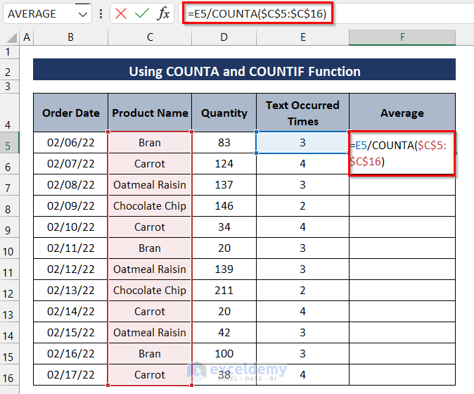
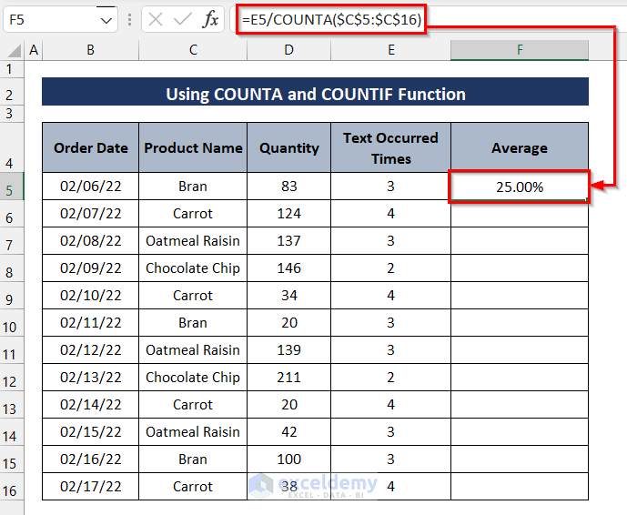
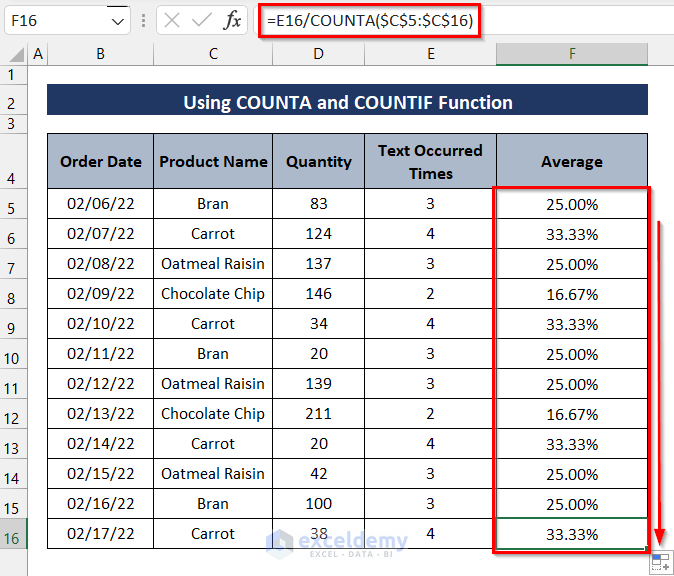
Thanks for your comment. I am replying to you on behalf of ExcelDemy. You can get the correct value by using the COUNTA function instead of the SUM function. Let’s see the steps.
Step-01: Write the following formula in the selected cell.
=E5/COUNTA($C$5:$C$16)Step-02: Press Enter to get the Average.
Step-03: Drag the Fill Handle down to copy the formula to the other cells.
I hope this will help you to solve your problem. Please let me know if you have other queries.
Regards
Mashhura,
ExcelDemy.
Hello Alun Vaughan-Evans,
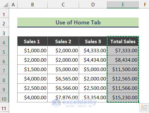
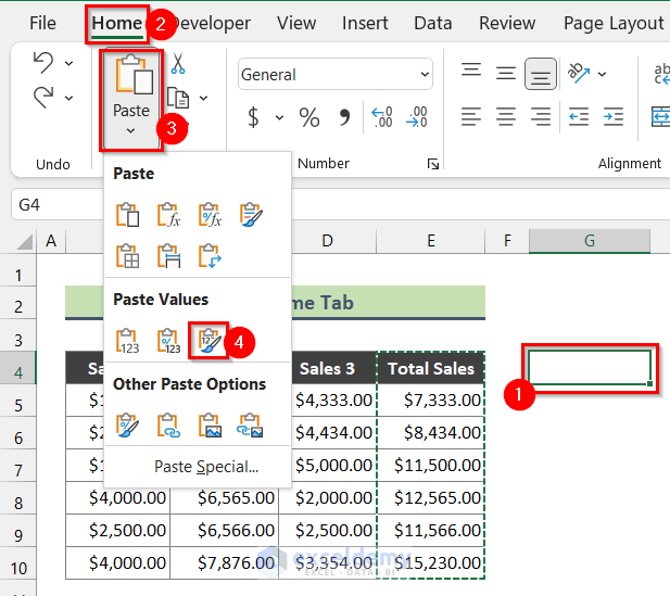
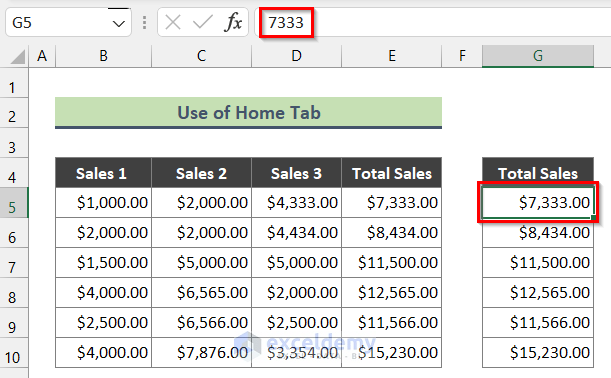
Thanks for your comment. I am replying to you on behalf of ExcelDemy. There is a way to keep the formatting and also values. You can follow these steps to do that.
Step-01: Select the range you want to copy and then copy the range by pressing Ctrl + C on your keyboard.
Step-02: Select the cell where you want to paste the range. And then go to Home > Paste > Values & Source Formatting (like the following image).
Finally, you will see that you have copied the values with formatting.
I hope this will help you to solve your problem. Please let me know if you have other queries.
Regards
Mashhura
ExcelDemy
Hello JC,
Thanks for your comment. I am replying to you on behalf of ExcelDemy. The downloaded file works for me.
You can follow the steps from the Feature of Eisenhower Matrix Template in Excel section. If it still doesn’t work then check if all cells contain the formula in the Eisenhower Matrix.
And, while making your own Eisenhower Matrix, check if you are applying for the same range as in this article. If not, change your ranges accordingly in the formula.
Lastly, if you are using an older version of Microsoft Excel then press Ctrl + Shift + Enter while entering the formula.
I hope this will help you to solve your problem. If none of these works then you can let us know at [email protected] with your Excel file and problem details. We will try our best to solve your problem.
Regards
Mashhura
ExcelDemy
Hi SEM,
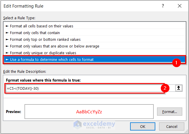
Thanks for your comment. I am replying to you on behalf of ExcelDemy. If you want to filter dates older than a number of days from today, you can follow the steps from Method-2. But, instead of the formula used here, write the following formula.
=C5<(TODAY()-30)Here, I wrote the formula for dates older than 30 days from today. You can change the formula according to your preference.
I hope this will help you to solve your problem. Please let me know if you have other queries.
Regards
Mashhura
ExcelDemy
Hi Penny,
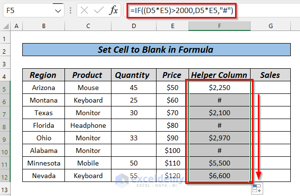
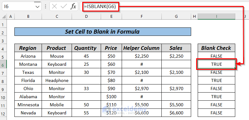
If you check to see if the cells are blank or not then they will be evaluated as not blank because the cells contain formula. If you need blank cells then you can follow these steps.
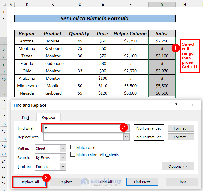
Step-01: In a Helper Column use any of the formulas from this article. But instead of an empty string (
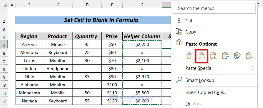
"") write a letter or a special character ("#") in the formula.=IF((D5*E5)>2000,D5*E5,”#”)Step-02: Copy the values from the Helper Column and Paste them as Values where you want the final output.
Step-03: Press Ctrl + H and the Find and Replace dialog box will appear. Replace # with nothing and you will get your blank cells.
Finally, if you check the cells, then you will see the cells are blank.
I have shared the necessary images for your convenience. I hope this will solve your problem. Please let me know if you have other queries.
Thanks!
Hello DQNOK,
Thank you for your feedback.
Hello Frank,
This article contains different methods for different situations. Method 1.3 hides the numbers that are less than Zero. But, if you want to hide zeros only then you can try the following code.
Option ExplicitSub Hide_Rows_With_Zero()Dim row As LongDim col As LongDim qq As BooleanFor row = 6 To 14qq = TrueFor col = 2 To 4If Cells(row, col).Value <> 0 Thenqq = FalseExit ForEnd IfNext colRows(row).Hidden = qqNext rowEnd SubI hope this will help you to solve your problem. Please let us know if you have other queries.
Thanks!