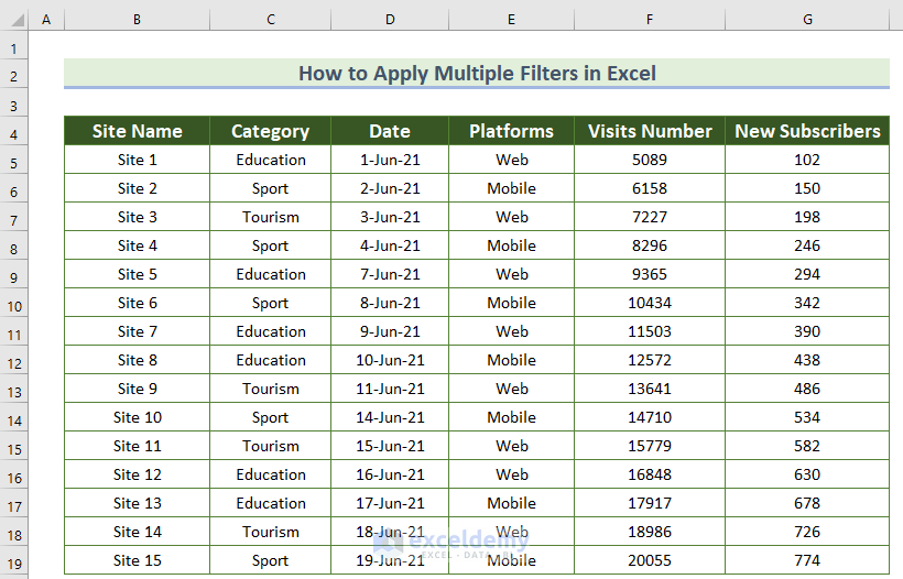
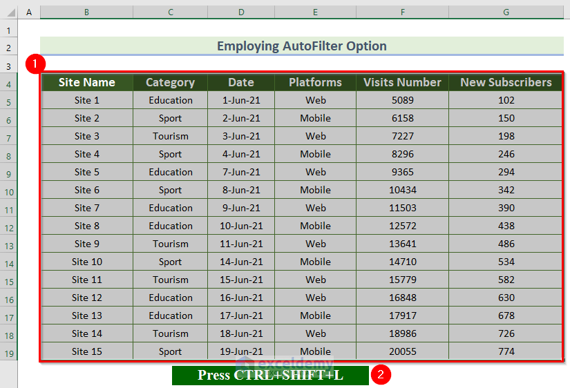
Before going to the steps, consider the following dataset. Here, the Names of 15 Sites are given along with their Category. Furthermore, the Visits Number and New Subscribers are provided based on the Date and mode of Platforms.
Now we’ll see the application of multiple filters regarding different perspectives. For conducting the session, we are using Microsoft 365 version. So, let’s get started.
Method 1 – Multiple Filters in Simple Way within Different Columns in Excel
If you want to get the number of visits for the Educational sites and the Mobile platform, you can simply use the Filter option.
Follow the steps below:
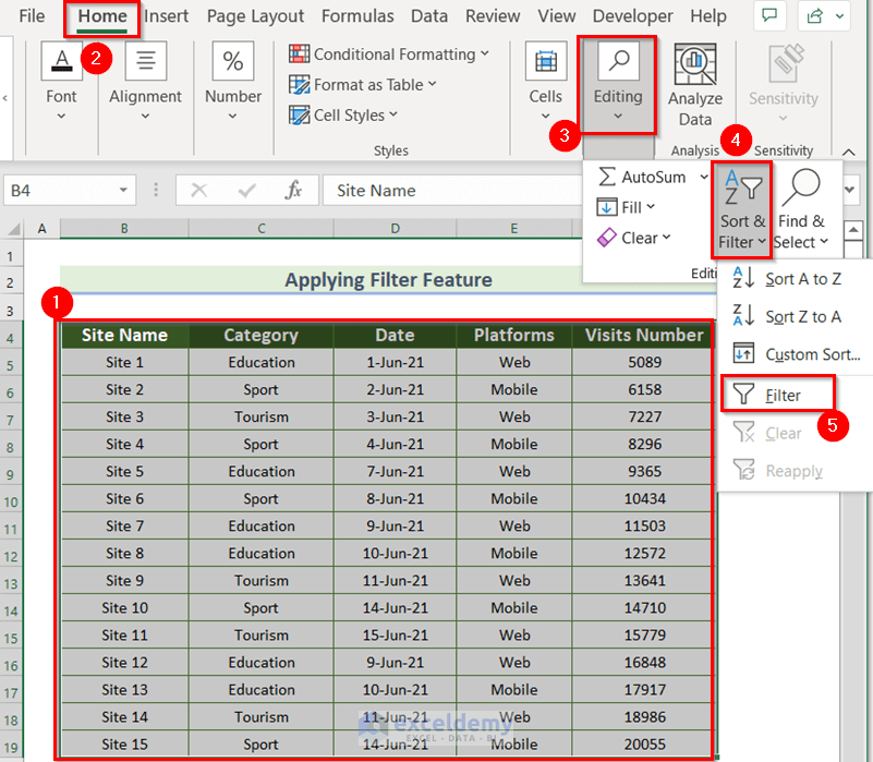
- Select your dataset.
- From the Home tab, click the Filter option (from the Sort & Filter command bar). Alternatively, go to the Data tab and click Filter.
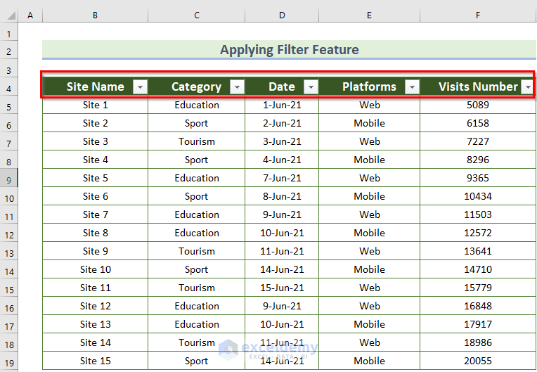
- After that, you’ll see the drop-down arrow for each field.
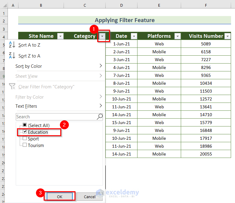
- Select the “Category” field.
- Uncheck the box close to Select All to deselect all the data options.
- Check the box close to “Education”.
- Press OK.
- Click on the “Platforms” field and check the box for “Mobile”
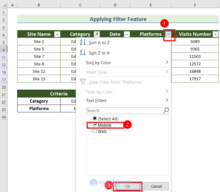
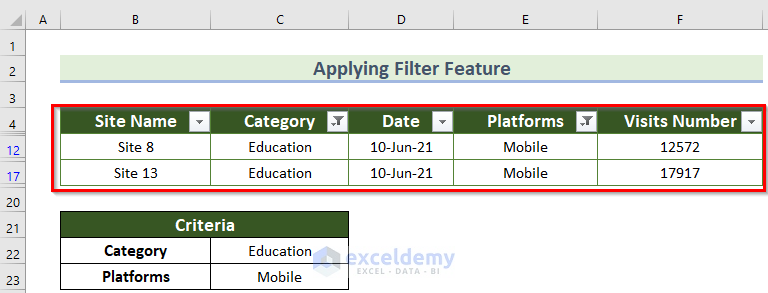
After filtering the two fields, you’ll get the following visits number.
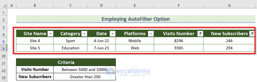
Method 2 – Using AutoFilter Option to Filter Multiple Values in Excel
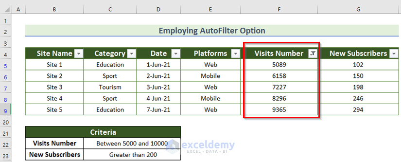
Let’s find the “Site Name” with a visits number between 5,000 and 10,000, where “New subscribers” are greater than 200.
- Select the dataset and press Ctrl + Shift + L.
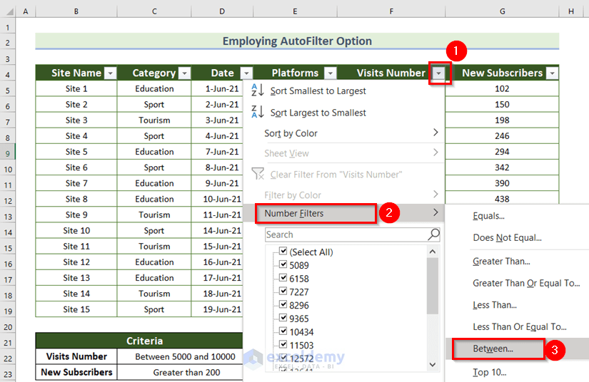
- Click on the drop-down arrow of the “Visits Number” field.
- Go to the Number Filters menu.
- Choose the Between option.
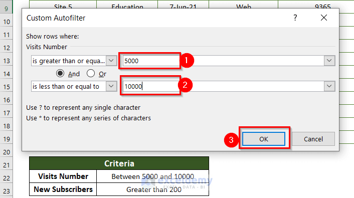
At this time, a new dialog box named Custom Autofilter will appear.
- Insert 5000 in the first blank space of the Custom AutoFilter dialog box.
- Write 10000 in the second space.
- Press OK.
- You will see the filtered Visits number.
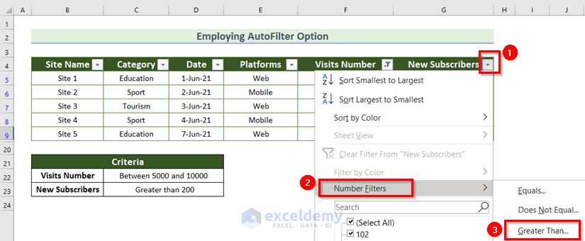
- Click on the drop-down arrow of the “New Subscribers” field.
- Go to the Number Filters menu.
- Choose the Greater Than option.
- In the dialog box named Custom Autofilter for “New subscribers” opens, put 200 in the top right box (next to “is greater than”).
- Press OK.
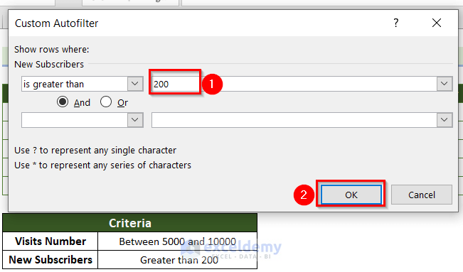
- And you’ll get the following result for your query.
Method 3 – Filter Multiple Columns Simultaneously Using Advanced Filter Feature
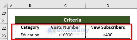
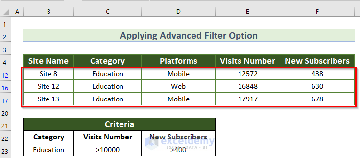
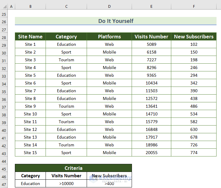
Let’s specify three criteria: category of the sites should be education, the number of visits being greater than 10,000, and the number of new subscribers needs to be greater than 400.
- Create a small table to detail the criteria. We have used cell range B22:D23. You must put the criteria horizontally. Note that the criteria headers must match those of the main table.
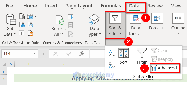
- Open the Advanced Filter option by going to the Data tab and clicking on Sort & Filter, then Advanced.
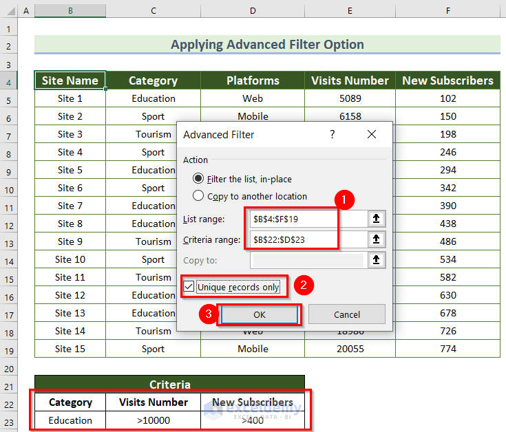
- Specify the range of your whole dataset from where you want to filter in the List range option and provide the criteria in the Criteria range.
- If you don’t need duplicates, check the box next to Unique records only.
- Press OK.
And you’ll see the following output.
Method 4 – Multiple Filters Employing VBA in Excel
Method 4.1. Multiple Filters Using OR Operator (Logic)
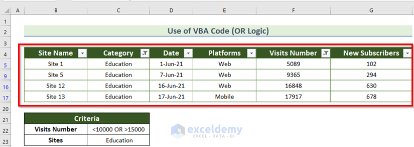
Suppose you need to shows websites with visits less than 10000 or greater than 15000, and the category of the sites would be education. Use these steps:
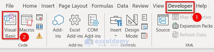
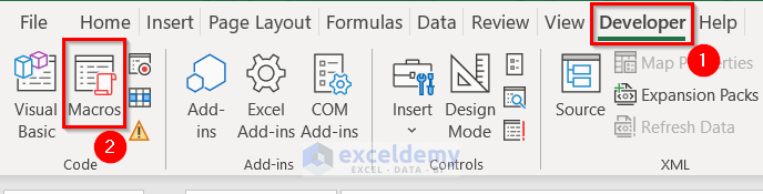
- From the Developer tab, click on Visual Basic.
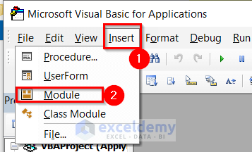
- Open a module by clicking on Insert, then Module.
- Copy the following code in Module 1.
Sub filter_my_sites()
Dim range_to_filter As Range
Set range_to_filter = Range("B4:G19")
range_to_filter.AutoFilter field:=5, Criteria1:="<10000", Criteria2:=">15000", Operator:=xlOr
range_to_filter.AutoFilter field:=2, Criteria1:="Education"
End Sub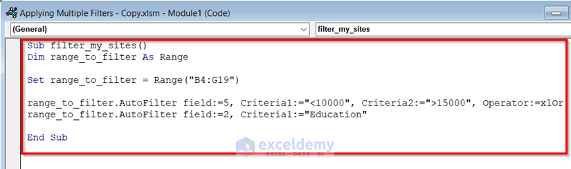
Code Breakdown
The following things are necessary for using the VBA AutoFilter.
- Range: It refers to the cell range to filter e.g. B4:G19.
- Field: It is the index of the column number from the leftmost part of your dataset. The value of the first field will be 1.
- Criteria 1: The first criteria for a field e.g. Criteria1=”<10000”
- Criteria 2: The second criteria for a field e.g. Criteria2=”>15000”
- Operator: An Excel operator that specifies certain filtering requirements e.g. Operator:=xlOr, Operator:=xlAnd, etc.
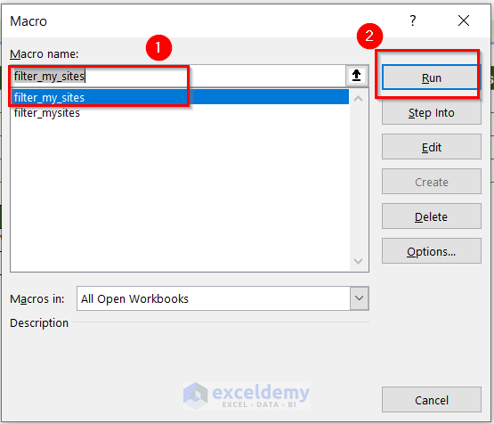
- From the Developer tab, go to Macros.
- Choose filter_my_sites from the Macro name and press Run.
If you run the above code, you’ll get the following output.
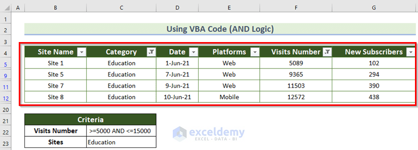
Method 4.2. Multiple Filters Using AND Operator (Logic)
To get the educational sites having a number of visits between 5000 and 15000, you may use the following code:
Sub filter_mysites_2()
Dim range_to_filter As Range
Set range_to_filter = Range("B4:G19")
range_to_filter.AutoFilter field:=5, Criteria1:=">=5000", Criteria2:="<=15000", Operator:=xlAnd
range_to_filter.AutoFilter field:=2, Criteria1:="Education"
End Sub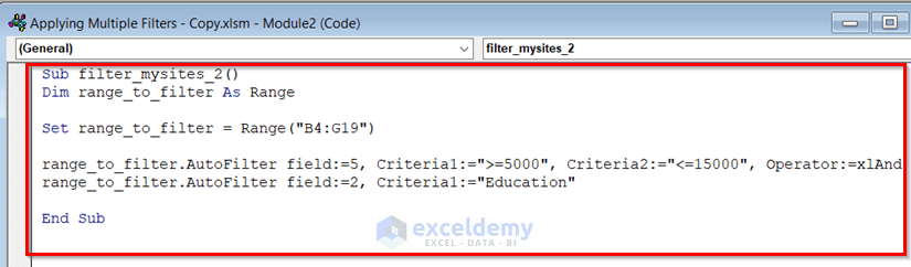
- After running the code, you’ll get the following output.
Method 5 – Use of FILTER Function to Apply Multiple Filters
This function only exists in the Excel 365 version, web version, and Excel 2021 and newer.
The syntax of the function is:
The arguments are-
- array: Range or array to filter.
- include: Boolean array, supplied as criteria.
- if_empty: Value to return when no results are returned. This is an optional field.
Suppose you want to filter the whole dataset for only the month of June. That means you want to get the name of sites, the number of visits, etc. for June.
- Write the formula in the H5 cell. Here, you should keep enough space for the filtered data otherwise it will show some error.
=FILTER(B5:F19,MONTH(D5:D19) > 5,"No data")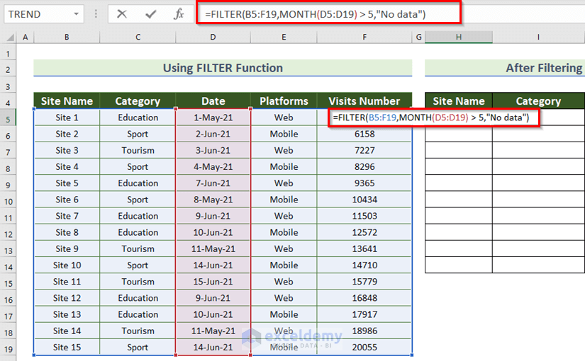
Here, B5:F19 is our dataset, D5:D19 is for the date, the syntax MONTH(D5:D19) > 5 returns the date for June.
- Press ENTER.
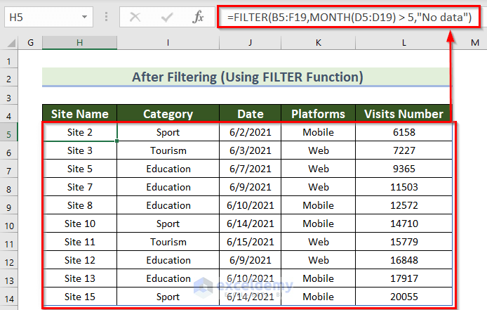
And, you’ll get the following output.
Method 6 – Use of Excel Table to Apply Multiple Filters
Steps:
- Select the data range.
- From the Insert tab, choose the Table feature.
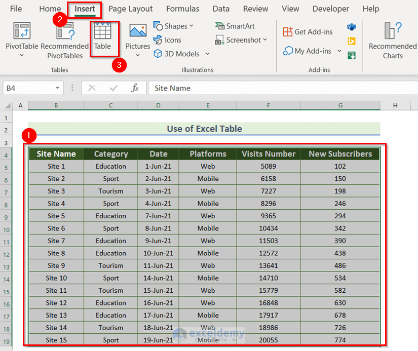
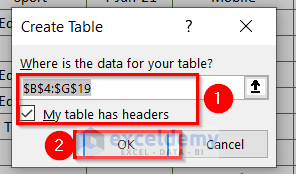
- A dialog box named Create Table will appear. Select the data range in the Where is the data for your table? box. Here, if you select the data range before then this box will auto-fill.
- Check the My table has headers option.
- Press OK.
- You’ll see the drop-down arrow for each field.
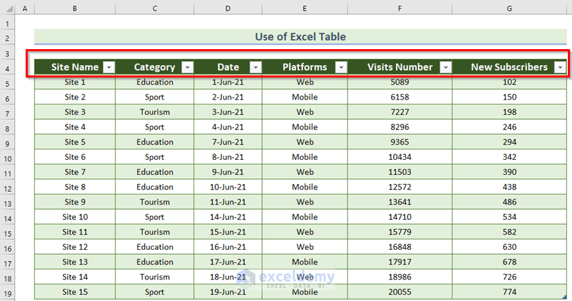
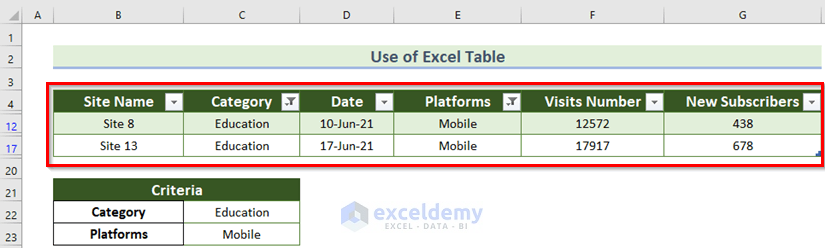
- Then, follow the steps of method 1 and you will get the output.
How to Filter Multiple Comma Separated Values in Excel
For this section, we will use a different data table, containing the Site Name, Category, Visits Number, and Platforms columns.
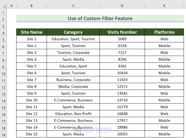
Let’s get the number of visits for the Educational sites and the Mobile platform:
- Select the dataset and press CTRL+SHIFT+L. You’ll see the drop-down arrow for each field.
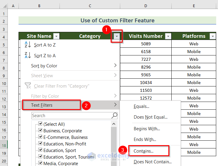
- Click on the drop-down arrow of the “Category” field.
- Go to the Text Filters menu.
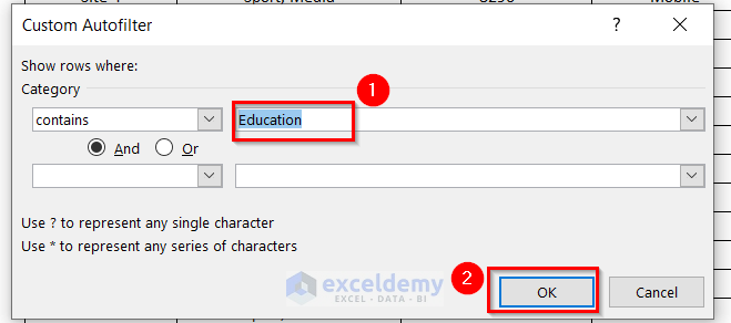
- Choose the Contains.. option. A new dialog box named Custom Autofilter will appear.
- Write Education in the first space (for “contains“).
- Press OK.
So, you will see the Category is filtered.
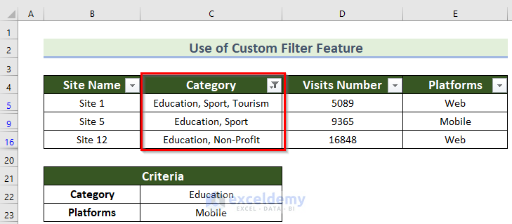
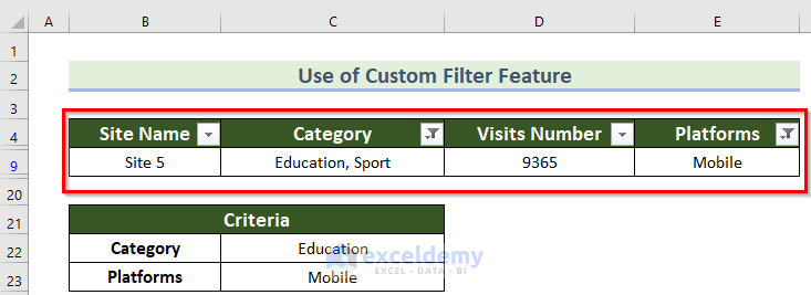
For filtering Platforms, follow method 1 and you will get the final output.
Practice Section
You can practice filtering by yourself via the provided sample.
Download Practice Workbook
You can download the practice workbook from here:


So beautiful manner to explain and to make understanding….
Thanks a lot…..
Hello Abdul Quadir Ali,
You are most welcome and thank you so much for your kind words! I’m so glad you found the explanation helpful and easy to understand. Your feedback truly means a lot!
Regards
ExcelDemy