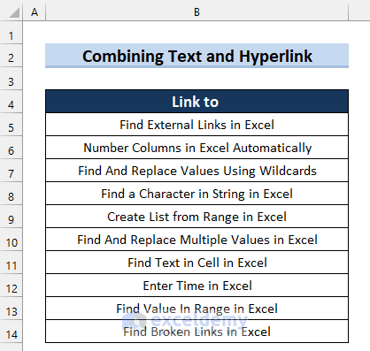
Before jumping into the methods, let’s learn about the dataset for this article. It contains some texts for web pages or documents, which will be used as the basis for inserting hyperlinks.
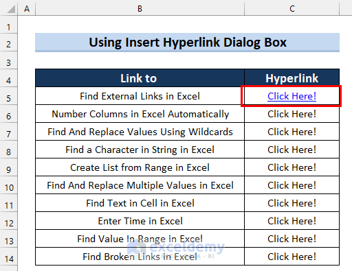
Method 1 – Use Insert Hyperlink Dialogue Box to Combine Text and Hyperlink in Excel
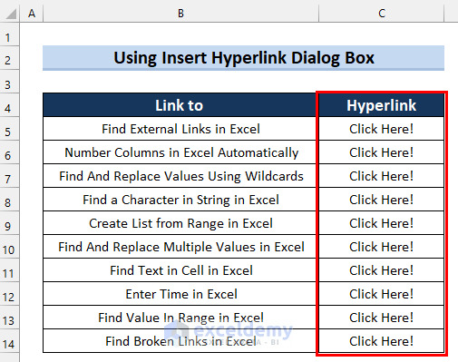
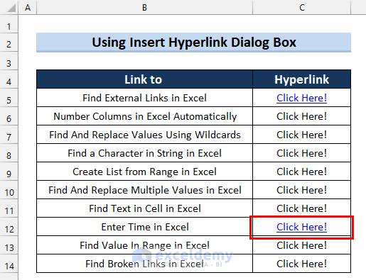
Let’s put the hyperlinks adjacent to the cell texts.
Steps:
- Create a column for Hyperlink.
- Fill the cells of the column with the text you want. We used “Click Here!”.
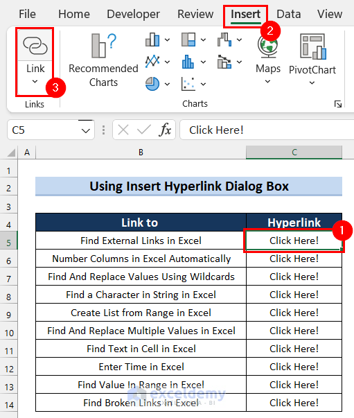
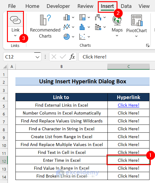
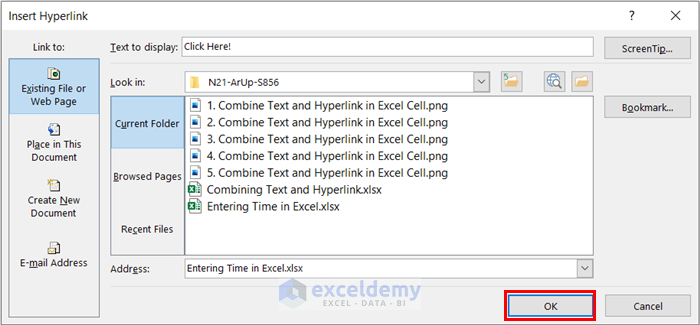
- Select cell C5.
- Go to the Insert tab.
- Select Link. The Insert Hyperlink dialog box will appear.
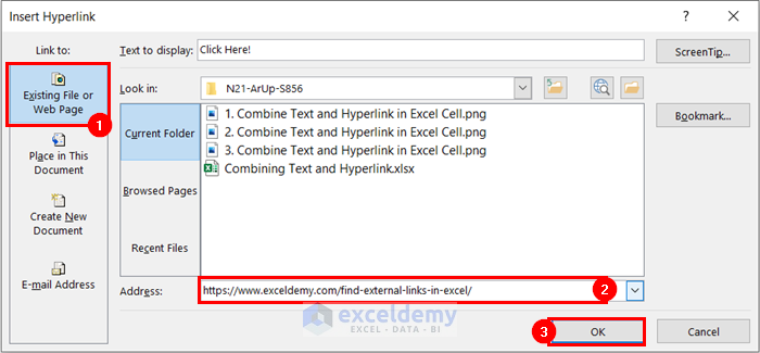
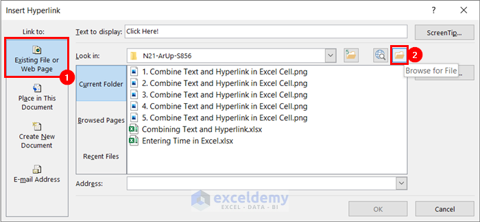
- Select Existing File or Web Page in the Link to section.
- Copy and paste the link for the web page as the Address.
- Select OK.
- You will see that you have combined a hyperlink to the selected text.
Let’s combine hyperlink and text for another Excel workbook from this computer:
- Select the cell where you want to combine the hyperlink with text.
- Go to the Insert tab.
- Select Link. The Insert Hyperlink dialog box will appear.
- Select Existing File or Web Page in the Link to section.
- Select Browse for File.
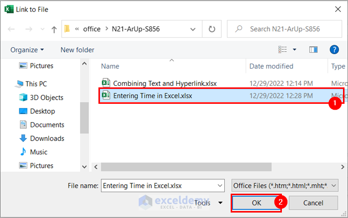
- Choose the file you want to link to.
- Hit OK.
- Select OK in the Insert Hyperlink dialog box to confirm.
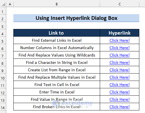
- You can see that a hyperlink is combined with the text.
- Repeat for the other cells.
- To check if a link works, click on the text.
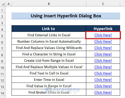
- Finally, you can see that the web page or sheet has opened for the selected text.
Read More: How to Create a Hyperlink in Excel
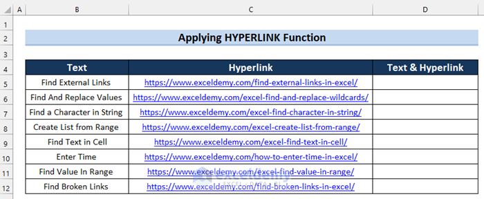
Method 2 – Apply HYPERLINK Function to Combine Text and Hyperlink in Excel Cell
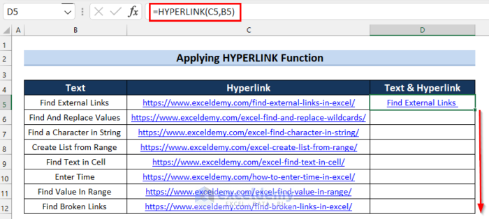
Let’s modify the dataset so it has 3 columns, Text, Hyperlink, and Text & Hyperlink. We will combine the text and hyperlink in the 3rd column.
Steps:
- Select D5.
- Write the following formula in that selected cell.
=HYPERLINK(C5,B5)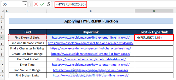
- Press Enter to get the result.
Here, in the HYPERLINK function, I selected Cell C5 as link_location, and Cell B5 as friendly_name. The formula will combine the text with the hyperlink.
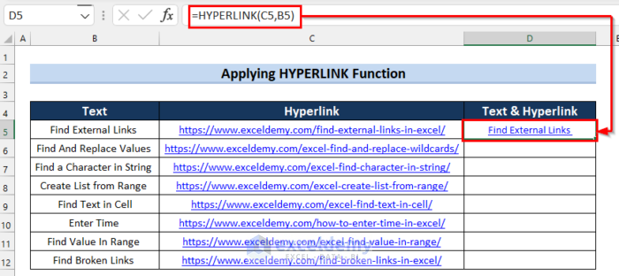
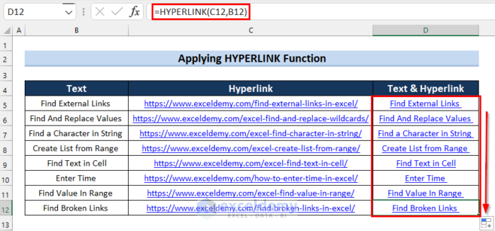
- Drag the Fill Handle down to copy the formula to the other cells.
- Excel has combined text and hyperlinks for all the other cells.
Read More: Excel Hyperlink with Shortcut Key
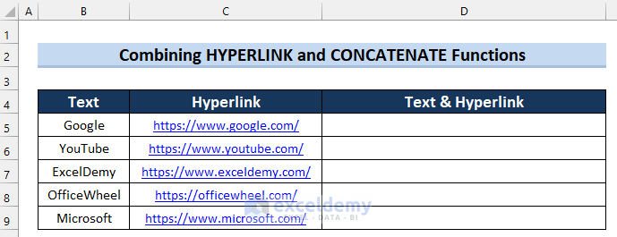
Method 3 – Combine HYPERLINK and CONCATENATE Functions to Join Text and Hyperlink in Excel Cell
Let’s use a similar dataset to display the text and link side-by-side in a cell.
Steps:
- In cell D5, write the following formula.
=HYPERLINK(C5,CONCATENATE(B5," Link: ",C5))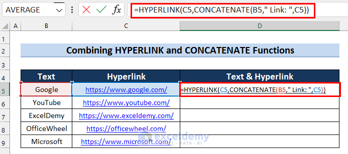
- Press Enter to get the output.
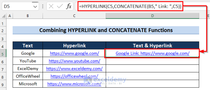
How Does the Formula Work?
- CONCATENATE(B5,” Link: “,C5): Here, in the CONCATENATE function, I selected Cell B5 as text1, ” LInk: ” as text2, and Cell C5 as text3. The formula will join these 3 texts.
- HYPERLINK(C5,CONCATENATE(B5,” Link: “,C5)): Now, in the HYPERLINK function, I selected Cell C5 as link_location, and CONCATENATE(B5,” Link: “,C5) as fiendly_name. The formula will combine the text and hyperlink and then jump into the selected location when you click on it.
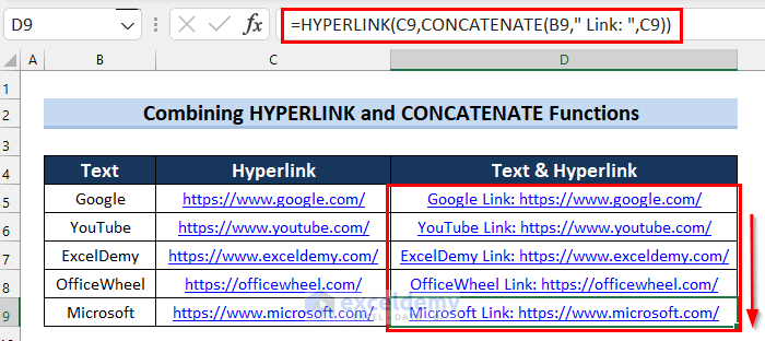
- Drag the Fill Handle down to copy the formula to the other cells.
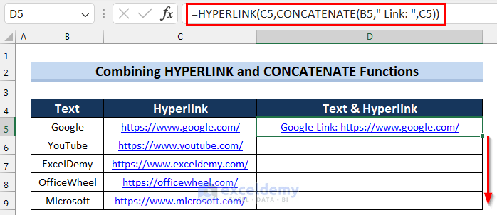
- Excel copied the formula to all the other cells.
Read More: How to Convert Text to Hyperlink in Excel
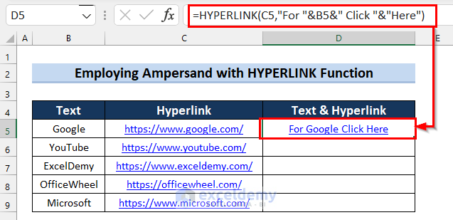
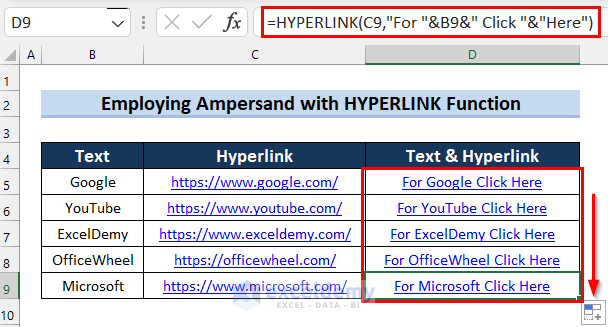
Method 4 – Employ Ampersand with HYPERLINK Function to Merge Text and Hyperlink in Excel Cell
Steps:
- Copy the following formula into D5.
=HYPERLINK(C5,"For "&B5&" Click "&"Here")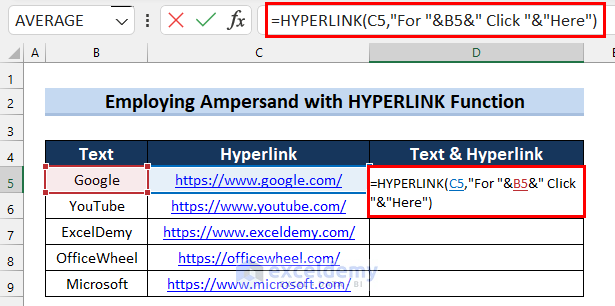
- Press Enter to get the result.
How Does the Formula Work?
- “For “&B5&” Click “&”Here”: Here, the Ampersand operator (&) joins these texts.
- HYPERLINK(C5,”For “&B5&” Click “&”Here”): Now, in the HYPERLINK function, I selected Cell C5 as link_location, and “For “&B5&” Click “&”Here” as fiendly_name. The formula combines the text and hyperlink and then jumps into the selected location when you click on it.
- Drag the Fill Handle down to copy the formula to the other cells.
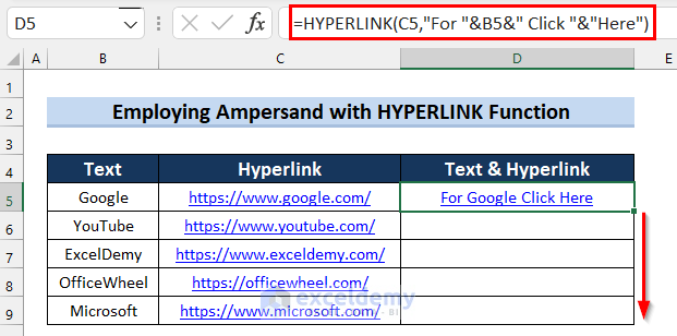
- Excel will fill the formula to the cells.
Read More: How to Find and Replace Hyperlinks in Excel
Things to Remember
- You need to use the HYPERLINK function to create a link in the text.
Download Practice Workbook
Download this practice sheet to practice while you are reading this article.
Similar Articles for You to Explore
- How to Hyperlink to Cell in Same Sheet in Excel
- Excel Hyperlink to Cell in Another Sheet with VLOOKUP
- How to Add Hyperlink to Another Sheet in Excel
- Excel Hyperlink to Another Sheet Based on Cell Value
- How to Create a Drop Down List Hyperlink to Another Sheet in Excel
- How to Edit Hyperlink in Excel
- How to Create Dynamic Hyperlink in Excel
- How to Copy Hyperlink in Excel
- How to Create Button to Link to Another Sheet in Excel
<< Go Back To Hyperlink in Excel | Linking in Excel | Learn Excel
Get FREE Advanced Excel Exercises with Solutions!
