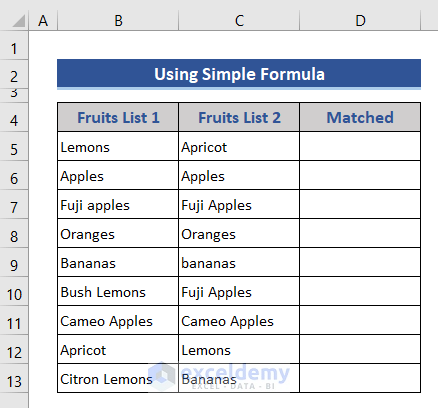
Method 1 – Use “Equal to” Operator to Compare Text Two Cells in Excel (Case Insensitive)
For this method let’s consider a dataset of fruits. In the dataset, we will have two columns for Fruits List. Our task is to match the names of the fruits and show their matched result.
Steps:
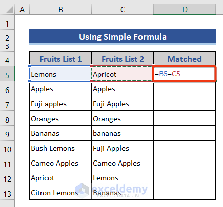
- Enter the following formula in Cell D5.
=B5=C5
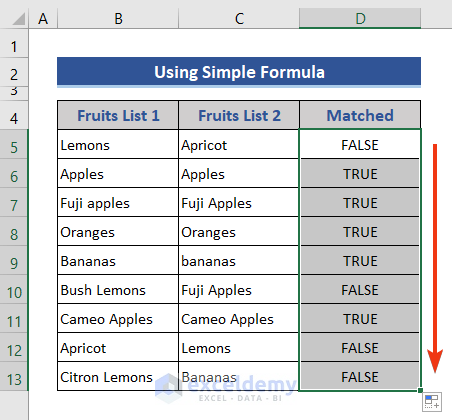
- Copy down the formula up to D13.
Note:
This formula will not work for case-sensitive issues that is why if the text matches with values but they are not in the same letter it will show TRUE for that.
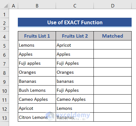
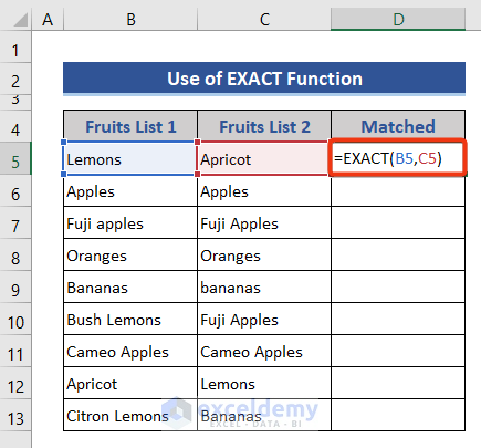
Method 2 – Apply Excel EXACT Function to Compare Two Cells’ Text (Case Sensitive)
For this method let’s use the same dataset as we used for Method 1. Our task is to compare the names of the fruits and show their exact matched result.
Steps:
- Enter the below formula in Cell D5.
=EXACT(B5,C5)
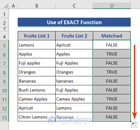
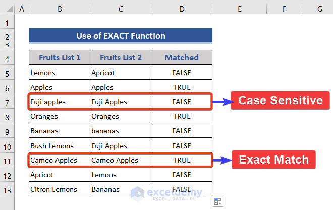
- Copy down the formula to D13.
Observation:
If you observe the result you can see that the EXACT function is returning the result TRUE if, and only if, the whole text is fully matched. It is also case-sensitive.
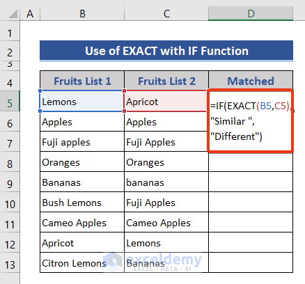
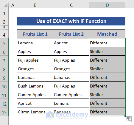
Use of EXACT Function with IF to Get a Text Output:
Steps:
- Enter the following formula in Cell D5.
=IF(EXACT(B5,C5),"Similar","Different")
Formula Explanation:
Our inner function is EXACT, which is going to find the exact match between two cells:
=IF (logical_test, [value_if_true], [value_if_false])
In the first portion, it takes the condition or criteria, then the value which will be printed if the result is true and then if the result is false.
We will print Similar if the two cells get matched and Different if they are not. That’s why the second and third argument is filled up with this value.
- Copy down the formula to D13.
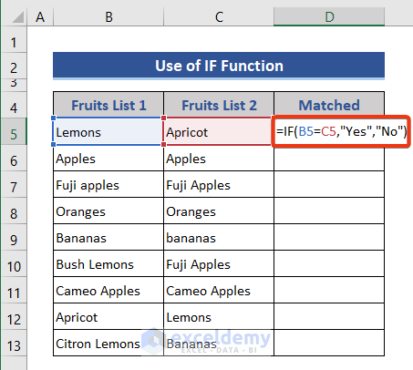
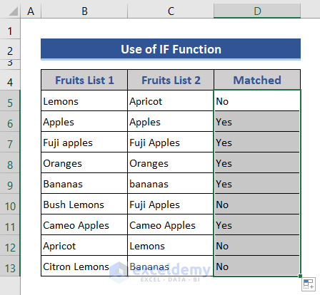
Method 3 – Insert Excel IF Function to Compare Text of Two Cells (Not Case-Sensitive)
Steps:
- Enter the below formula in Cell D5.
=IF(B5=C5,"Yes","No")
- Copy down the formula up to D13.
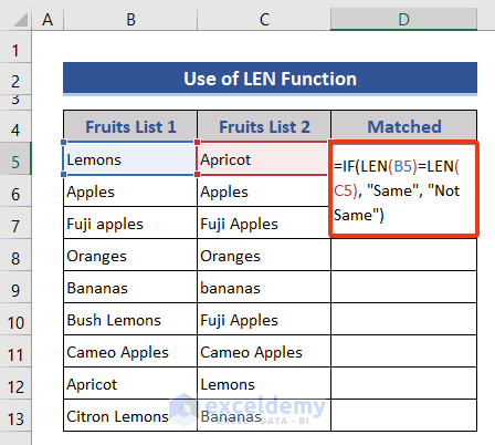
Method 4 – Compare Text of Two Cells by String Length with Excel LEN Function
This method looks for the same length of text, rather than the same text. Our dataset will be the same as above.
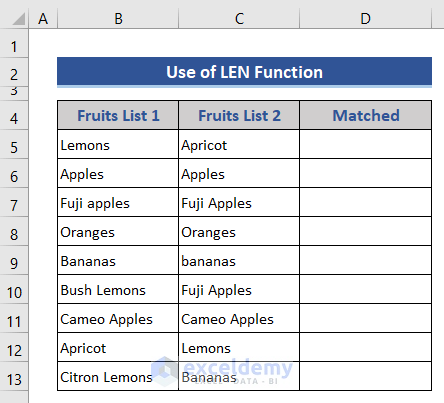
Steps:
- Enter the below formula in Cell D5.
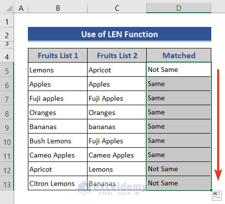
=IF(LEN(B5)=LEN(C5), "Same", "Not Same")
Formula Explanation:
- This function is used to count the characters of any text or string. When we pass any text in this function, it will return the number of characters.
- LEN(B5) this part first counts the character of each cell from the first column and LEN(C5) for the second one.
- If the length is the same then it will print the “Same” and if not then “Not Same”.
- Copy down the formula up to D13.
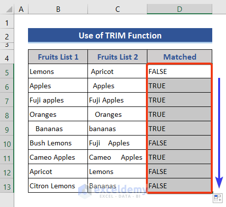
Method 5 – Compare Two Cells Containing Text That Have Unnecessary Spaces in Excel
Using the same dataset we’ve used for the previous methods, let’s find out which results have the same text after removing spaces.
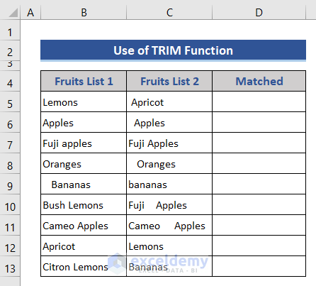
Steps:
- Enter the formula below in Cell D5.
=TRIM(B5)=TRIM(C5)
Formula Explanation:
- The syntax of this function is: TRIM(text). This function is used to remove all spaces from a text string except for single spaces between words.
- TRIM(B5) this part removes unnecessary spaces from the cell expect single spaces between words and TRIM(C5) for the second one.
- After removing spaces if both are the same then it will print the “TRUE” and if not then “FALSE”.
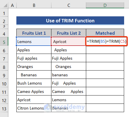
- Copy down the formula up to D13.
Method 6 – Compare Text Strings of Two Cells in Excel by Occurrences of a Specific Character
For this method, we will see how to compare two cells by the Occurrence of a Specific Character. Let’s consider a dataset of products with their send ID and received ID. These ids are unique and should be matched with send and receive IDs. We want to make sure that each row contains an equal number of shipped and received items with that specific ID.
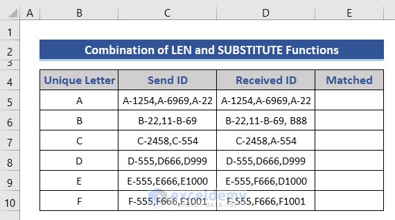
Steps:
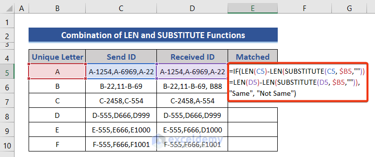
- Enter the below formula in Cell E5.
=IF(LEN(C5)-LEN(SUBSTITUTE(C5, $B5,""))=LEN(D5)-LEN(SUBSTITUTE(D5,$B5,"")),"Same","Not Same")
Formula Explanation:
- We have used the SUBSTITUTE function, which has the following fundamentals
- The syntax of this function is: SUBSTITUTE (text, old_text, new_text, [instance])
- These four arguments can be passed in the function’s parameter, with the last one being optional:
text- The text to switch.
old_text- The text to substitute.
new_text- The text to substitute with.
instance- The instance to substitute. If not provided, all instances are replaced. - SUBSTITUTE(B2, character_to_count,””) using this part we are replacing the unique identifier with nothing using the SUBSTITUTE function.
- Then using LEN(C5)-LEN(SUBSTITUTE(C5, $B5,””)) and LEN(D5)-LEN(SUBSTITUTE(D5, $B5,””)) we are calculating how many times the unique identifier appears in each cell. For this, get the string length without the unique identifier and subtract it from the total length of the string.
- Lastly, the IF function is used to make the results more meaningful for your users by showing the true or false results.
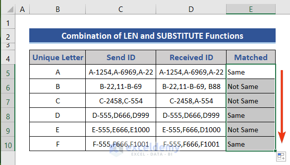
- Copy down the formula up to E10.
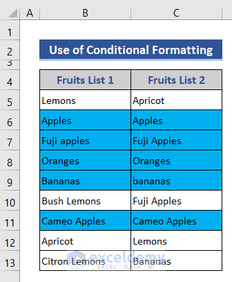
Method 7 – Highlight Matches by Comparing Text from Two Cells in Excel
Steps:
- Select the entire dataset.
- Go to Conditional Formatting under the Home tab.
- Select the New Rule option.
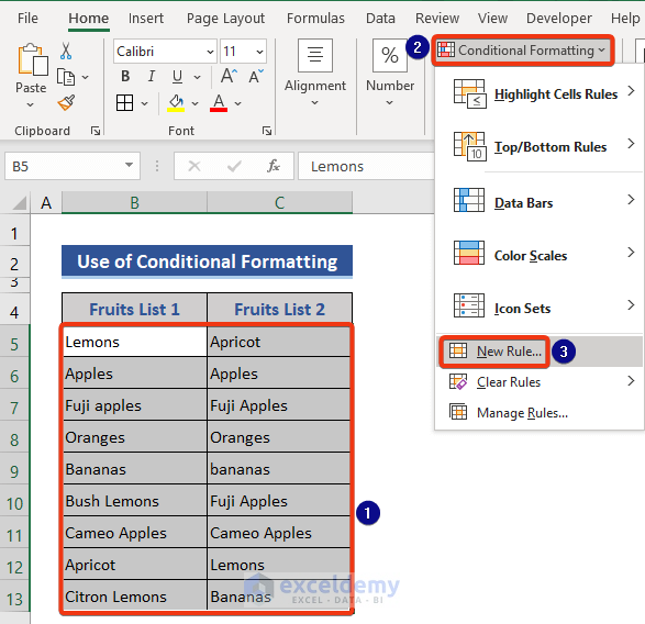
- Select the option marked 1.
- Enter the below formula in the marked box 2.
=$B5=$C5
- Or you can just select the two columns of the dataset.
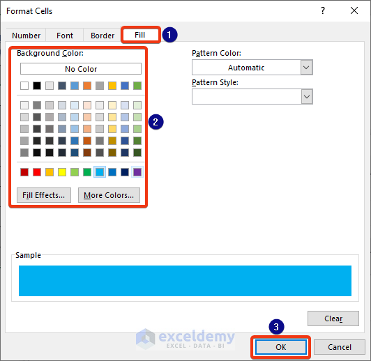
- Click on the Format option.
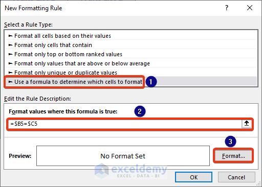
- Go to the Fill tab.
- Select any color.
- Press OK.
- Click the OK button.
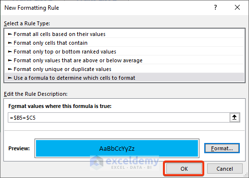
- See the matched data highlighted.
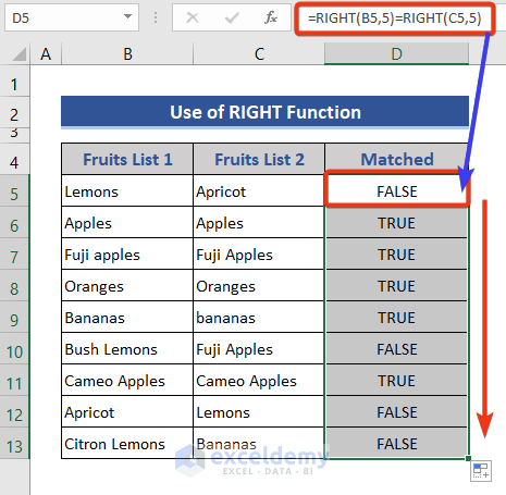
Method 8 – Compare Text from Two Cells Partially in Excel (Not Case-Sensitive)
For this method, we’ll use the below data table to find if the last 6 characters are matched across two cells.

Steps:
- Enter the below formula in Cell D5 and copy down the formula up to
=RIGHT(B5,5)=RIGHT(C5,5)
Method 9 – Find Matched Text in Any Two Cells in Same Excel Row
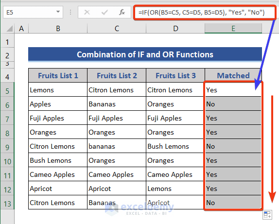
Let’s have a dataset of three fruit lists. Now we will compare the cells one with each other and we get any two cells matched in the same row then it will be considered as matched.
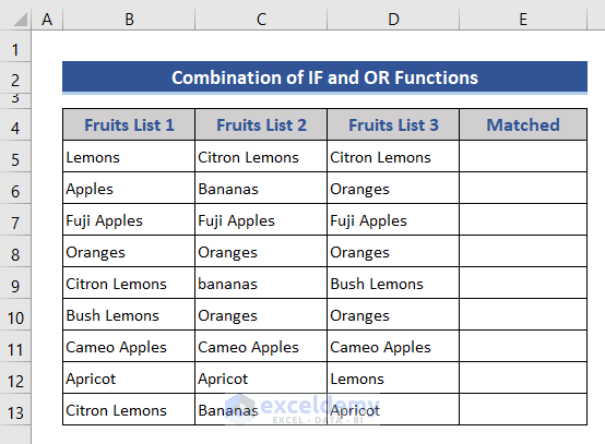
Steps:
- Enter the formula in Cell E5 and copy down the formula up to
=IF(OR(B5=C5,C5=D5,B5=D5),"Yes","No")
Formula Explanation:
- You have used the OR function here, which has the following syntax – OR (logical1, [logical2], …)
- It can take two or more logics in its parameters.
logical1 -> The first requirement or logical value to decide.
logical2 -> This is optional. The second requirement or logical value to evaluate. - OR(B5=C5, C5=D5, B5=D5)
This portion decides if all the cells are equal or at least two are equal or not. If yes then the IF function decides the final value based on the OR function’s result.
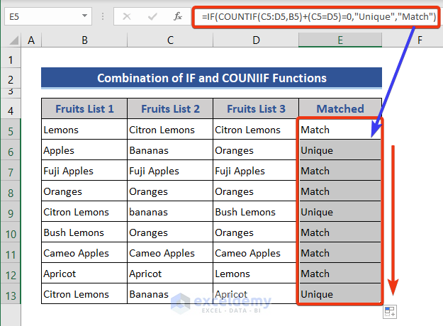
Method 10 – Find Unique and Matched Cells by Comparing Text of Multiple Cells
Steps:
- Enter the below formula in Cell E5 and copy down the formula up to
=IF(COUNTIF(C5:D5,B5)+(C5=D5)=0,"Unique","Match")
Formula Explanation:
- Here the COUNTIF function is used.
- In this function both the arguments in the parameter are mandatory. Firstly, it takes the range of cells that will be counted. The second section takes the criteria which is the condition. Counting is executed based on this condition.
- By using COUNTIF(C5:D5,B5)+(C5=D5)=0 we are trying to find out if the row has matched or unique values. If the count is 0 then it is unique otherwise there is a matched value.
How to Compare One Cell with an Entire Column in Excel
Here, we have a dataset with one fruit list and a matching cell. Now we will compare the matching cell with the Fruit List column and find the match result.
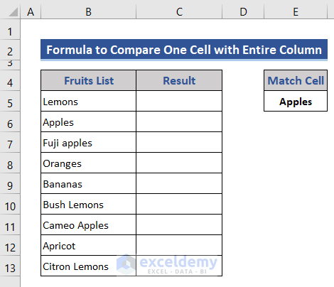
Steps:
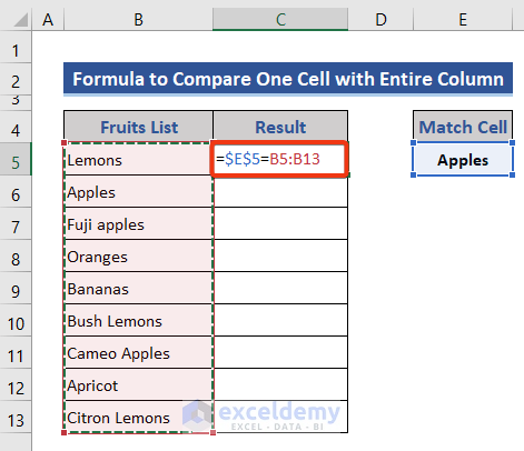
- Enter the below formula in Cell E5.
=$E$5=B5:B13
- Press the Enter button.
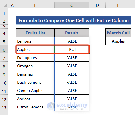
When Cell E5 matches with corresponding cells of Range B5:B13, then returns TRUE. Otherwise, it returns FALSE.
Download Practice Workbook
<< Go Back To Excel Compare Cells | Compare in Excel | Learn Excel
Get FREE Advanced Excel Exercises with Solutions!
