How to Paste in Reverse Order in Excel

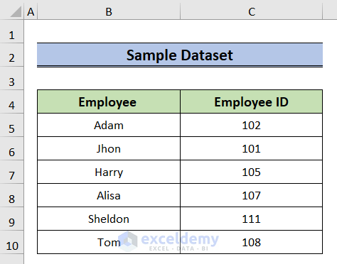
How to Paste in Reverse Order in Excel – 7 Methods

The following is the sample dataset.

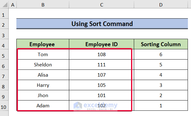
Method 1 – Using the Sort Command

1.1 Pasting in Reverse Order Vertically

Steps:

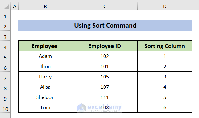
Select D5 cell and enter 1.

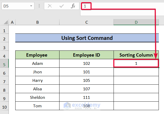
Enter numeric values in the subsequent cells in ascending order.
Here, 1 to 6.

Go to the Data tab on the ribbon.
Choose Sort & Filter.
Select Sort Largest to Smallest.

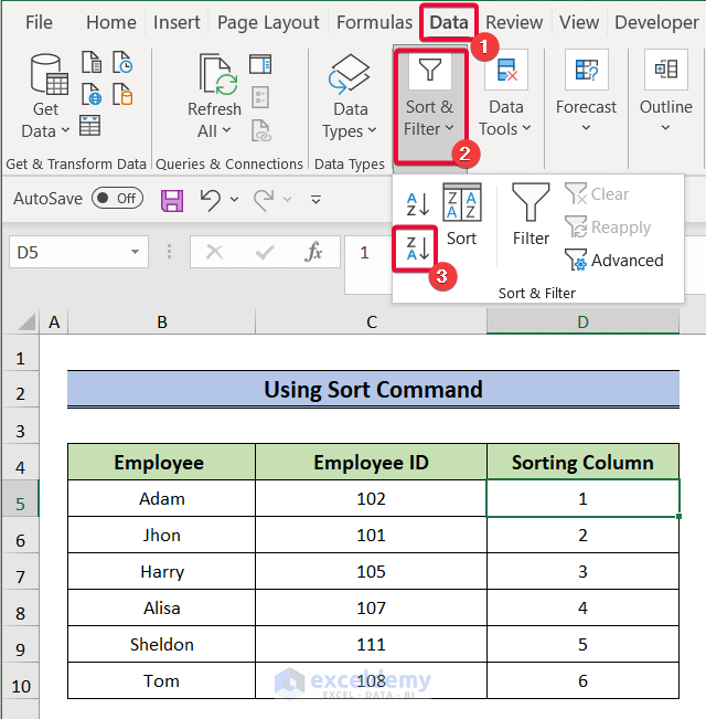
The data order will be reversed.

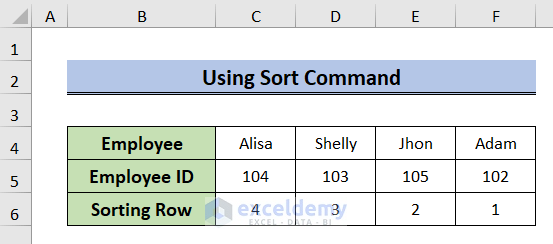
1.2 Pasting in Reverse Order Horizontally

Steps:

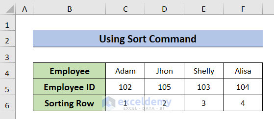
Enter 1 in C6.

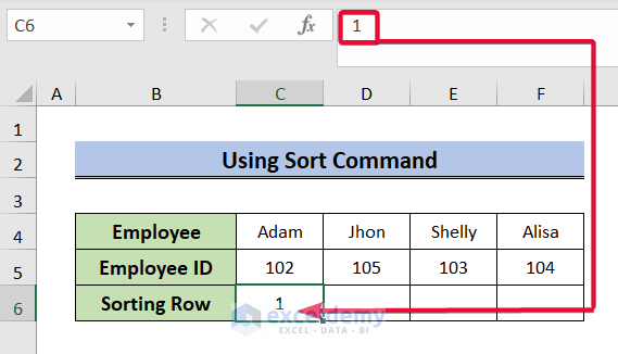
Enter numbers in ascending order from the left to the right.
Here, 1 to 4.

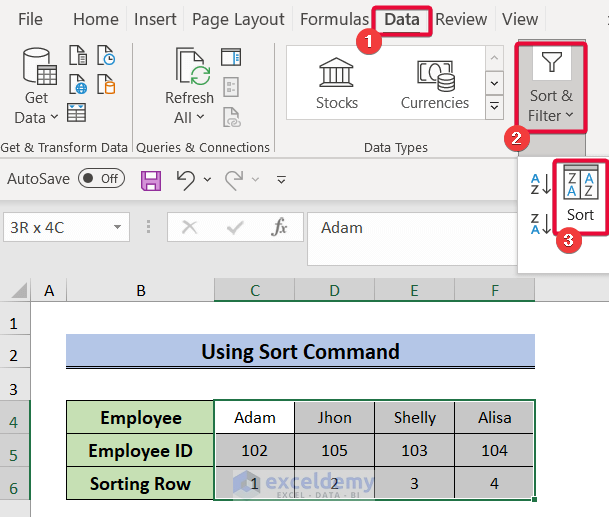
Select the dataset and go to the Data tab on the ribbon.
Choose Sort & Filter.
Select Sort.

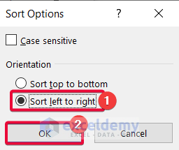
Select Options.

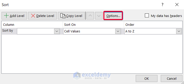
Select Sort left to right in Sort Options.
Click OK.

Go back to Sort prompt and select Sort by. Row 6, here.
Choose Largest to Smallest as the Order.
Click OK.

The dataset will be in reverse order.

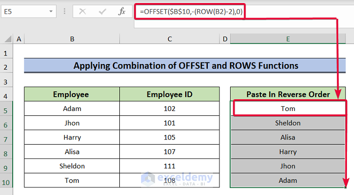
Method 2 – Combining OFFSET and ROW Functions

Steps:

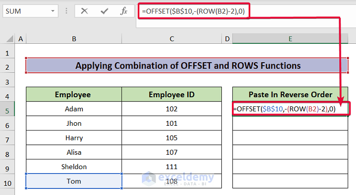
Select E5 and enter the following formula,

=OFFSET($B$10,-(ROW(B2)-2),0)

Press Enter.

Data is pasted in reverse order.
Drag the Fill Handler across the cells you want to fill.

Formula Breakdown:

(ROW(B2)-2): The ROW function takes B2 as a reference and returns 2 (the number of the cell). 2 is then subtracted from the cell and returns zero.
OFFSET($B$10,-(ROW(B2)-2),0): The OFFSET function takes B10 as a reference. The two arguments – rows and cols – define how many rows and columns to move from the reference cell. As both rows and cols arguments have zero values, the function returns the value in B10, which is Tom. On the other hand, in the next cell the ROW function holds B3 as a reference, so it will return 3. If we subtract 2 from 3, the value is 1. The rows argument of the OFFSET function will be -1. The OFFSET function will return the value of the cell above the reference cell, which is Sheldon.

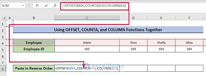
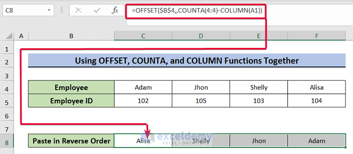
Method 3 – Using the OFFSET, COUNTA, and COLUMN Functions Together

Steps:

Select C8 cell and enter the following formula.

=OFFSET($B$4,,COUNTA(4:4)-COLUMN(A1))

Press Enter.

Data is pasted in reverse order.
Drag the Fill Handler across the cells you want to fill.

Formula Breakdown:

COLUMN(A1): The Column function takes A1 as a reference and returns 1 which is the column number of the cell.
COUNTA(4:4): The COUNTA function counts the number of non-empty cells in a given range. In this case, the number of non-empty cells in the 4:4 range is 5.
OFFSET($B$4,,COUNTA(4:4)-COLUMN(A1)): The OFFSET function takes B4 as a reference. The two arguments- rows and cols– define how many rows and columns to move from the reference cell. Here, the rows argument is empty. The cols argument is COUNTA(4:4)-COLUMN(A1) which returns, 5-1 or 4. The OFFSET function will return 4, the number of cells to the right of B4. In this case, Alisa.

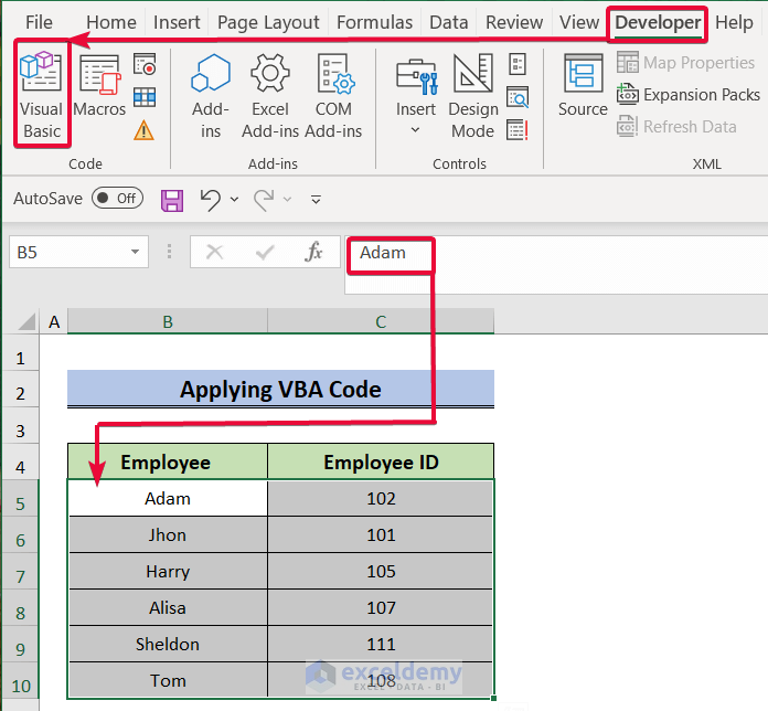
Method 4 – Applying a VBA Code

4.1 Pasting in Reverse Order Vertically

Steps:

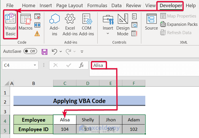
Select the dataset.
Go to the Developer tab on the ribbon.
Select the Visual Basic toolbar.

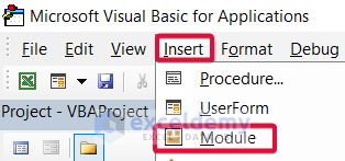
In the Visual Basic tab, click Insert.
Select Module.

In the coding module, enter the following code and save it.

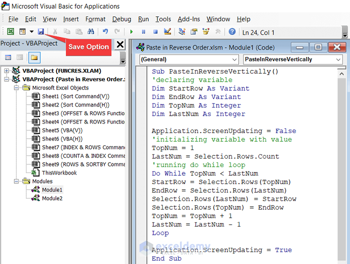
Sub PasteInReverseVertically()
'declaring variable
Dim StartRow As Variant
Dim EndRow As Variant
Dim TopNum As Integer
Dim LastNum As Integer
Application.ScreenUpdating = False
'initializing variable with value
TopNum = 1
LastNum = Selection.Rows.Count
'running do while loop
Do While TopNum < LastNum
StartRow = Selection.Rows(TopNum)
EndRow = Selection.Rows(LastNum)
Selection.Rows(LastNum) = StartRow
Selection.Rows(TopNum) = EndRow
TopNum = TopNum + 1
LastNum = LastNum - 1
Loop
Application.ScreenUpdating = True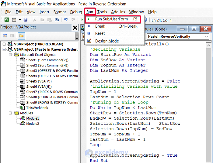
End Sub

Click the Run tab.
Select Run from the drop-down menu to run the code.

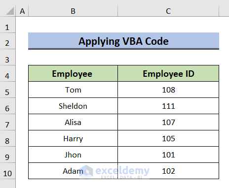
Data order is reversed.

4.2 Pasting in Reverse Order Horizontally

Steps:

Select the dataset.
Go to the Developer tab on the ribbon.
Select Visual Basic.

Click Insert.
Select Module.

Enter the following code and save.

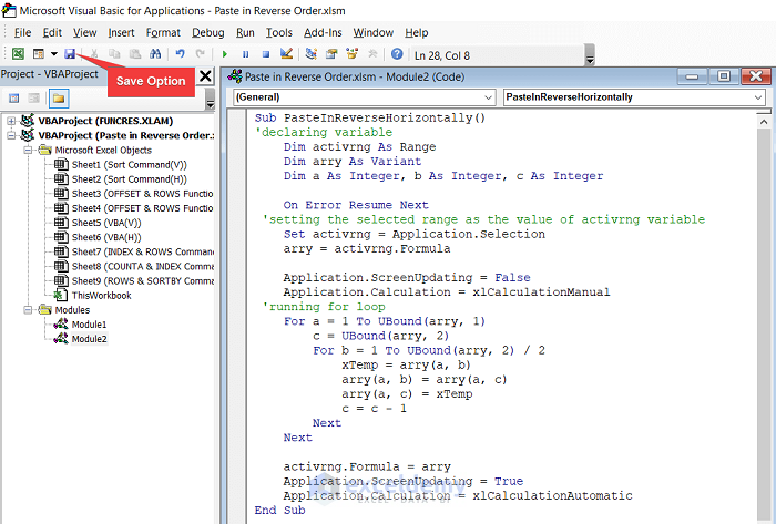
Sub PasteInReverseHorizontally()
'declaring variable
    Dim activrng As Range
    Dim arry As Variant
    Dim a As Integer, b As Integer, c As Integer
    On Error Resume Next
 'setting the selected range as the value of activrng variable
    Set activrng = Application.Selection
    arry = activrng.Formula
    Application.ScreenUpdating = False
    Application.Calculation = xlCalculationManual
 'running for loop
    For a = 1 To UBound(arry, 1)
        c = UBound(arry, 2)
        For b = 1 To UBound(arry, 2) / 2
            xTemp = arry(a, b)
            arry(a, b) = arry(a, c)
            arry(a, c) = xTemp
            c = c - 1
        Next
    Next
    activrng.Formula = arry
    Application.ScreenUpdating = True
    Application.Calculation = xlCalculationAutomatic
End Sub

Select the Run tab and click Run from the drop-down menu to run the code, .

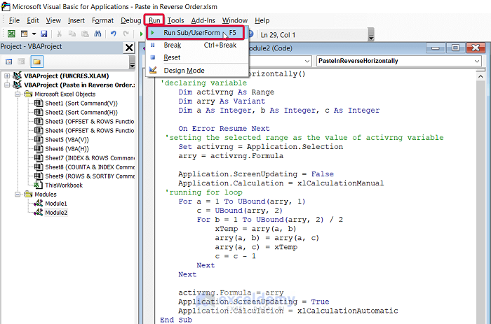
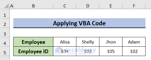
Data order has been changed.

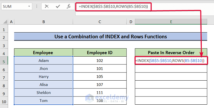
Method 5 – Combine INDEX and Rows Functions

Steps:

Select E5 cell and enter the formula below.

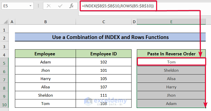
=INDEX($B$5:$B$10,ROWS(B5:$B$10))

Press Enter.

Data is pasted in the opposite order.
Drag the Fill Handler across the cells you want to fill.

Formula Breakdown:

ROWS(B5:$B$10): The ROWS function takes the B5:$B$10 range and returns the number of cells within that range. In this case, 6. Notice that B5 has relative cell reference and B10 has absolute cell reference. By moving down the cursor, B5 will be B6, but B10 will not change. So, the ROWS function will return 5.
INDEX($B$5:$B$10,ROWS(B5:$B$10)): The INDEX function will number the cells in the range B5:B10. B5 cell will be number 1 and in ascending order B10 cell will be number 6. When the ROWS function returns 6 in the ROWS(B5:$B$10) formula, the INDEX function takes it as the number of the row. The INDEX function will return the value in B10 which is Tom.

Read More: How to Reverse Rows in Excel

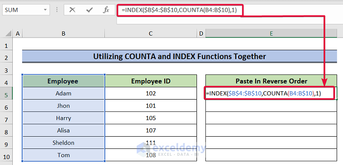
Method 6 – Using COUNTA and INDEX Functions Together

Steps:

Select E5 cell and enter the formula below.

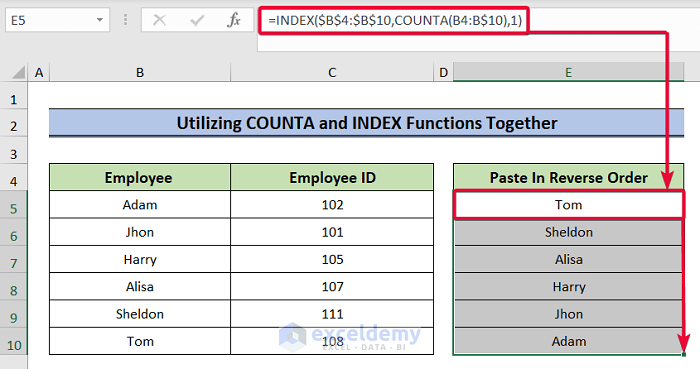
=INDEX($B$4:$B$10,COUNTA(B4:B$10))

Press Enter.

Data is pasted in the opposite order.
Drag the Fill Handler across the cells you want to fill.

Formula Breakdown:

COUNTA(B4:B$10): The COUNTA function counts the number of non-empty cells in the range B4:B$10. In this case, 7. Notice that B4 has relative cell reference and B10 has absolute cell reference. So, by moving down the cursor, B4 cell will be B5, but B10 cell will not change. So, the COUNTA function will return 6.
INDEX($B$4:$B$10,COUNTA(B4:B$10)): The INDEX function will number the cells in the range B4:B10. B4 will have 1 and in ascending order B10 will have 7. When the COUNTA function returns 7 in the COUNTA(B4:B$10) formula, the INDEX function takes it as the number of the row. The INDEX function will return the value in B10 which is Tom.

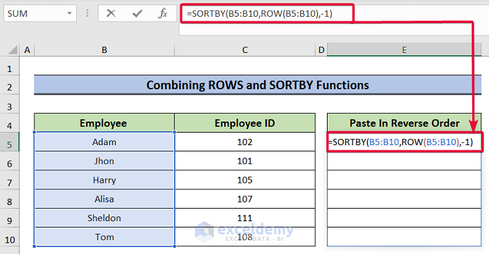
Method 7 – Combining ROW and SORTBY Functions

Steps:

Select E5 cell and enter the formula below.

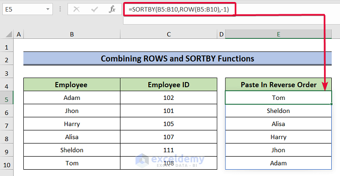
=SORTBY(B5:B10,ROW(B5:B10),-1)

Press Enter.

Data is pasted in reverse order.

Formula Breakdown:

ROW(B5:B10): The ROW function returns the number of rows in the range B5:B10.
SORTBY(B5:B10,ROW(B5:B10),-1): The SORTBY function’s first argument defines data that will be sorted. Here, the cell range B5:B10. The next argument is by_array1 which defines the array by which the previous array will be sorted. In this case, the array will be 1-6 which is returned by the ROW function. The next array is the sort_order1 which indicates in which order the array will be sorted. -1 indicates a reverse order.

How to Paste in Reverse Order in Excel – 7 Methods

How to Paste in Reverse Order in Excel – 7 Methods

Method 1 – Using the Sort Command

1.1 Pasting in Reverse Order Vertically

1.2 Pasting in Reverse Order Horizontally

Method 2 – Combining OFFSET and ROW Functions

Method 3 – Using the OFFSET, COUNTA, and COLUMN Functions Together

Method 4 – Applying a VBA Code

4.1 Pasting in Reverse Order Vertically

4.2 Pasting in Reverse Order Horizontally

Method 5 – Combine INDEX and Rows Functions

Method 6 – Using COUNTA and INDEX Functions Together

Method 7 – Combining ROW and SORTBY Functions

Related Articles

Leave a reply Cancel reply