The pie chart is one of the widely used charts in Excel. We use it for data presentation in a summarized way over a specific period of time. The colors in a pie chart help to determine each data point. These colors are easy to change in Excel. So in this article, we will learn how to change pie chart colors in Excel in 5 easy ways.
How to Change Pie Chart Colors in Excel: 4 Easy Ways
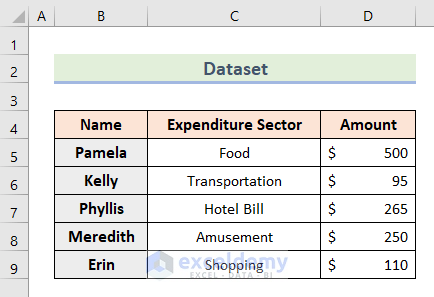
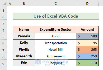
For illustration, we have taken a dataset as an example. The dataset shows expenditure sectors with amounts among 5 friends on a trip.
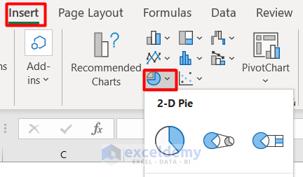
Now, select the dataset and create a Pie chart from the Charts group in the Insert tab.
Finally, we have our desired pie chart of expenses.

Now, let’s see 4 easy ways to change this pie chart’s colors in Excel.
1. Use Fill Color Tool to Change Pie Chart Colors
The Fill Color tool is an easy one to change the pie chart colors. Let’s see how it works.
- First, double-click on any of the slices in the pie chart.

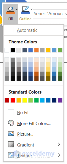
- Then, right-click and select Fill.
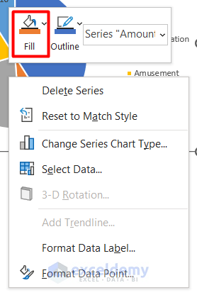
- After that, select any color you prefer for the slice.
- Finally, you can see that the selected slice color is changed now.

- Similarly, you can also change other slice colors by selecting them individually.
- You can find the similar Fill Color tool in the Font group of the Home tab.
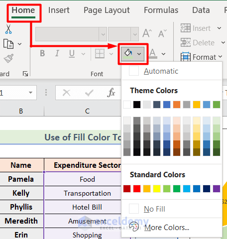
- If you want to explore an extensive range of colors, simply select More Colors below the color list.

- Here, in the Colors window, you have a wide range of colors to choose from for your pie chart.

2. Apply Themes in Excel to Modify Pie Chart Colors
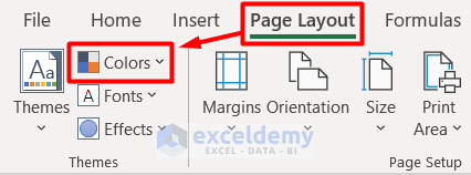
The Themes tool helps to change all slice colors of the pie chart at a time. Follow the steps below to perform this:
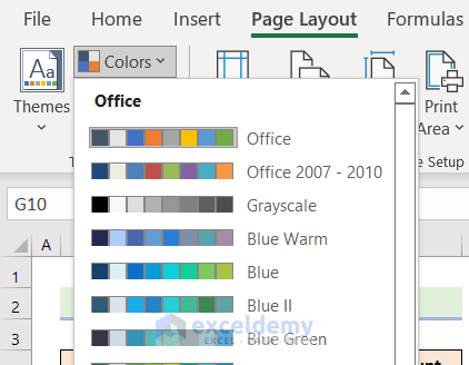
- To begin the process, select Colors in the Themes group of the Page Layout tab.
- Next, choose any color set you prefer for the pie chart.
- Finally, all the slice colors are changed at once in the Excel pie chart.

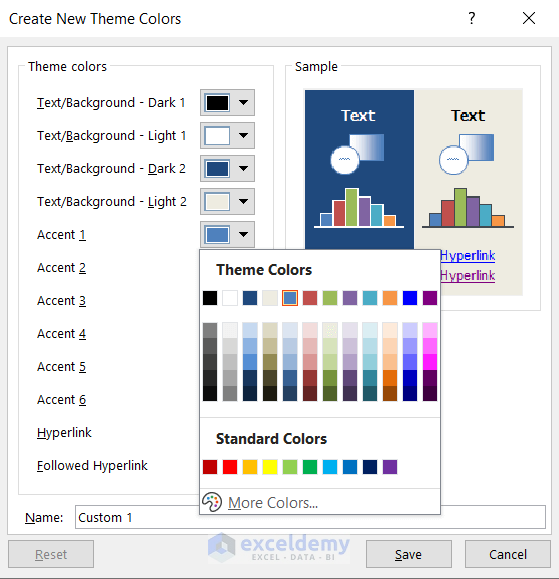
- To edit any color of the selected color set, go to Customize Colors below the color set options.
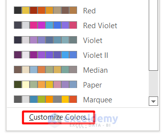
- Here, in the Create New Theme Colors window change any slice colors you want.
- Click on Save.
Read More: How to Edit Legend of a Pie Chart in Excel
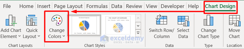
3. Change Pie Chart Colors in Excel with Chart Style
In this section, we will discuss the process to change pie chart colors with the Chart style. Let’s see the steps below:
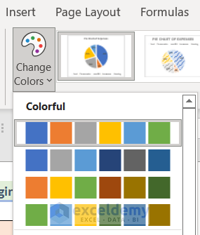
- First, choose Change Colors under the Chart Styles group in the Page Layout tab.
- After that, select any color set from the options in the drop-down section.
- That’s it, we have our newly colored pie chart in Excel.

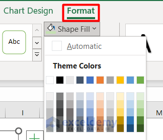
- To ornament it more, you can change the background color of the pie chart as well.
- Simply click on the Shape Fill icon under the Shape Styles group from the Format tab.
- Then, select any color you prefer for the background.
- Finally, here is the final output.

Read More: How to Edit Pie Chart in Excel
4. Use Excel VBA Code to Change Pie Chart Colors
In this last segment, we will change pie chart colors with Excel VBA code. Let’s follow the process below:
- First, color the cells D5:D9 manually with the Fill Color tool.
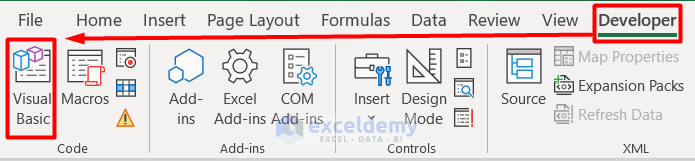
- Then, select Visual Basic from the Code group under the Developer tab.
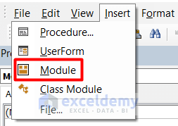
- Following, a new visual basic window appears.
- Here, select Module from the Insert tab.
- Now, insert the code below on the blank page.
Private Sub SheetActivate()
    Dim ch As ChartObject
    Dim l As Long
    Dim vntValues As Variant
    Dim st As String
    Dim myS As Series

    For Each ch In ActiveSheet.ChartObjects

        For Each myS In ch.Chart.SeriesCollection

            If myS.ChartType <> xlPie Then GoTo SkipNotPie

            s = Split(myS.Formula, ",")(2)
            vntValues = myS.Values

            For l = 1 To UBound(vntValues)
                myS.Points(l).Interior.Color = Range(s).Cells(l).Interior.Color
            Next l
SkipNotPie:
        Next myS
    Next ch
End Sub
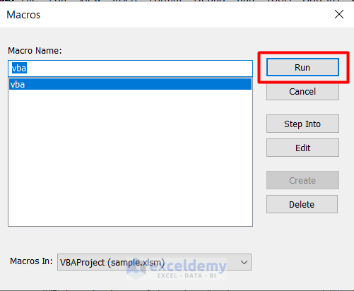
- After that, click on the Run Sub button or press F5 on your keyboard.

- Next, click on Run in the Macros window.
- Finally, you can see the pic chart color has changed according to the reference cells’ color.

Read More: Excel Pie Chart Labels on Slices: Add, Show & Modify Factors
How to Format Pie Chart Color in Excel
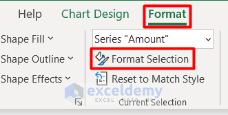
Here is a quick overview of how to format a pie chart color in Excel.
- First, double-click on any slice of your pie chart.
- Then, select Format Selection in the Current Selection group under the Format tab.
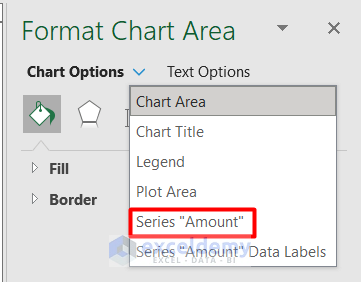
- After that, choose Series “Amount” among the Chart Options in the Format Chart Area pane.
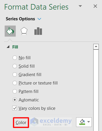
- Now, change the Color from this section.
- You can do this for each slice if it is necessary.
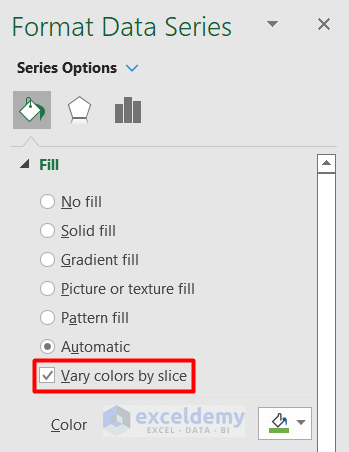
- Keep the Vary colors by slice option checked if you want different colors in each slice.
- Otherwise, mark it unchecked to keep all the colors the same.
- Explore the Format Chart Area pane for more pie chart modification options.
Read More: Add Labels with Lines in an Excel Pie Chart
Download Workbook
Conclusion
In this article, we tried to guide you on how to change pie chart colors in Excel in 4 easy ways. We also went through some quick formatting tricks. Let us know if you can suggest more methods.
Related Articles
- How to Rotate Pie Chart in Excel
- How to Explode Pie Chart in Excel
- [Fixed] Excel Pie Chart Leader Lines Not Showing
- How to Hide Zero Values in Excel Pie Chart
<< Go Back To Edit Pie Chart in Excel | Excel Pie Chart | Excel Charts | Learn Excel
Get FREE Advanced Excel Exercises with Solutions!
