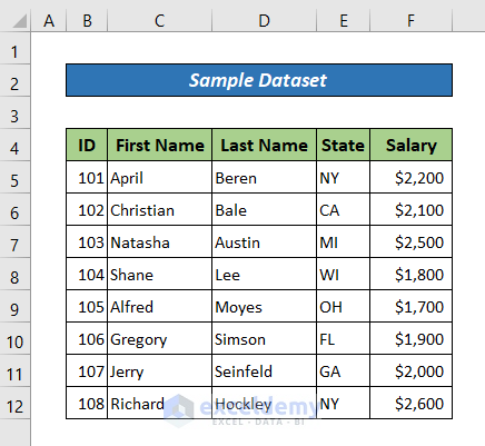
We have a dataset containing 5 columns and 9 rows including headings. Let’s extract data from this Excel worksheet to another worksheet.
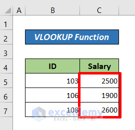
Method 1 – Extract Data from Excel Sheet Using VLOOKUP Function
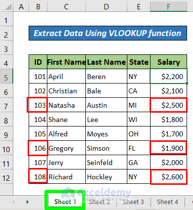
Suppose we need to extract the salaries of ID no. 103, 106, and 108 from sheet 1 to sheet 2.
Steps:
- Enter the following formula in Cell C13 of Sheet 2:
=VLOOKUP(B13,'Sheet 1'!B5:F12,5,FALSE)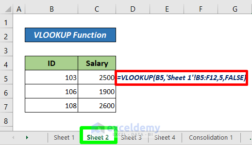
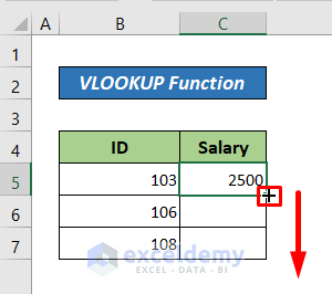
- Drag the Fill Handle to the range you need.
- Here is the output.
Note:
=VLOOKUP(lookup_value, table_array, col_index_num, [range_lookup])
Here,
- Lookup_value is the value you want to match
- Table_array is the data range that you need to look for your value
- Col_index_num is the corresponding column of the look_value
- Range_lookup is the boolean value (True or False). 0 (false) refers to an exact match and 1 (true) refers to an approximate match.
Read More: How to Extract Specific Data from a Cell in Excel
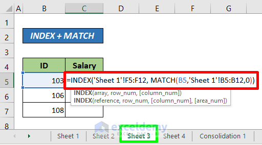
Method 2 – Pick Data from Excel Sheet Using INDEX-MATCH Formula
Suppose you want to find the salary for a particular ID.
Steps:
- In cell C13, enter the following formula:
=INDEX('Sheet 1'!F5:F12, MATCH(B13,'Sheet 1'!B5:B12,0))Here,
- MATCH(B13,’Sheet 1’!B5:B12,0) refers to cell B13 as the lookup_value in the data range B5:B12 for an exact match. It returns 3 because the value is in row number 3.
- INDEX(‘Sheet 1′!F5:F12, MATCH(B13,’Sheet 1’!B5:B12,0)) refers to Sheet 1 as an array of F5:F12 from where we will get the value.
- Press Enter.
- Drag the Fill Handle to the range you need.
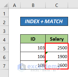
- Here is the output:

Read More: How to Extract Data Based on Criteria from Excel
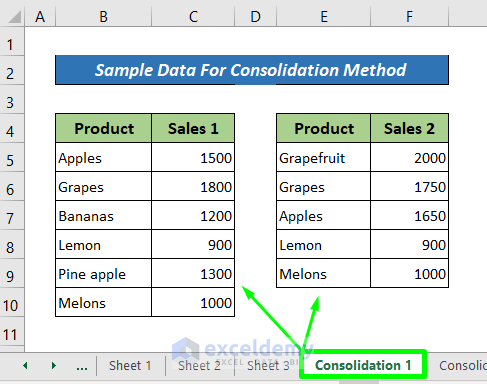
Method 3 – Extract Data from Excel Sheet Using Data Consolidation Tool
Let’s use two datasets in the same Excel worksheet (Consolidation 1) as input. The result of the consolidation will be shown on a different worksheet (Consolidation 2).
Steps:
- Go to the Consolidation 2 sheet and select a cell (Cell B4 in this example) where you want to put your consolidated result.
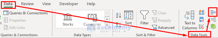
- Go to the Data tab, into the Data Tools group, and click on the Consolidate icon.
- A Consolidate Dialog box will pop up.
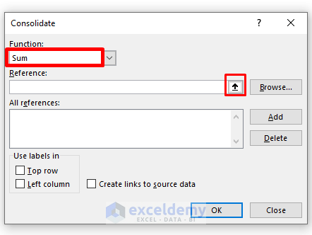
- Select the Function you need, then one by one select each table including the headings from the “Consolidation 1” sheet in the Reference box, and click Add.
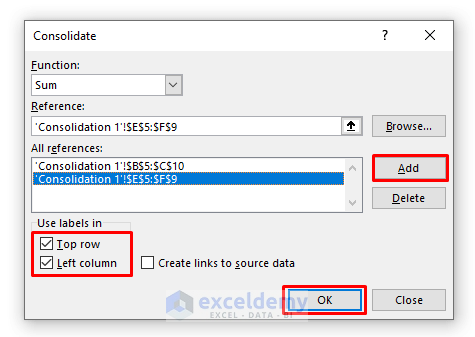
- All selected tables from Consolidation Sheet 1 will appear in the All References box. Check both Tick marks (top row and left row) in the Labels box.
- Click OK.
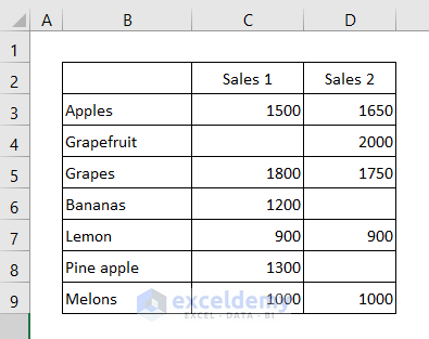
- Here is the result:
Read More: How to Extract Data From Table Based on Multiple Criteria in Excel
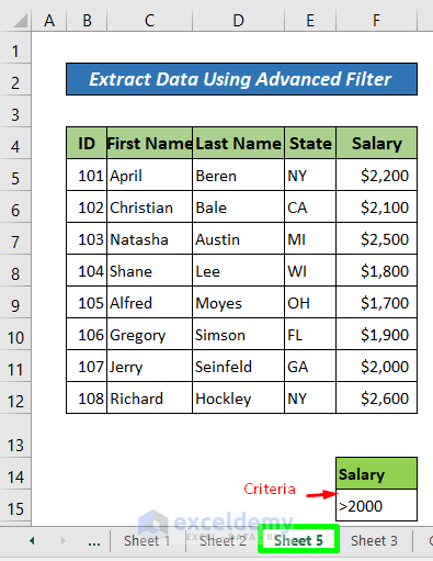
Method 4 – Extract Data from Worksheet Using Advanced Filter
In this example, the data is on Sheet 5 and will be extracted from Sheet 6.
Steps:
- Go to Sheet 6 and select a Cell (Cell B4 in this illustration).
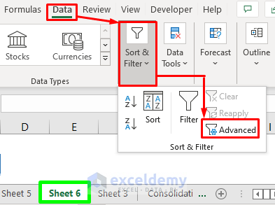
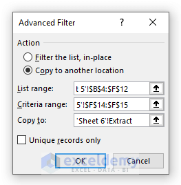
- Go to the Data tab, choose Sort & Filter, and click Advanced. An Advanced Filter window will open.
- Select Copy to Another Location.
- Click on the List Range box and select Sheet 5, then select the entire table with the headings.
- Choose the criteria range.
- In Copy to Box, select the cell on sheet 6 (Cell B4 in this example).
- Click OK.
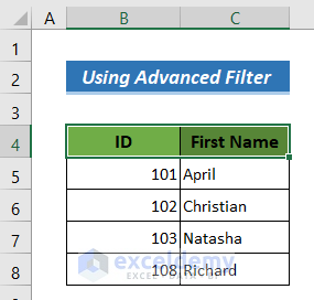
- Here is the result:
Read More: How to Extract Data from Cell in Excel
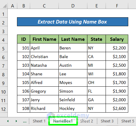
Method 5 – Pull Data from Another Sheet in Excel with the Help of Name Box
Suppose we have two worksheets named NameBox1 and NameBox2. We want to extract data from NameBox1 to NameBox2.
Steps:
- In any cell in NameBox2 (Cell B4 in this example), enter =NameBox1!C9 and press Enter and you will get values from Cell C9 in your new worksheet.
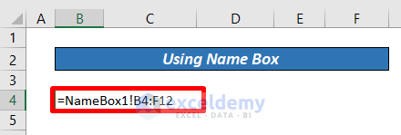
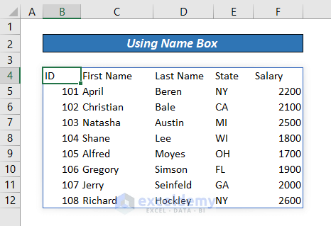
- Here is the result:
OR
- Type ‘=’ in any cell from NameBox2, then click the NameBox1 sheet and select the cell you need and press Enter.
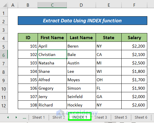
Method 6 – Extract Data from Excel Sheet with INDEX Function
Suppose we have two sheets named INDEX 1 and INDEX 2. In INDEX 2 sheet, we will set the Row and Column no. of the data from the INDEX 1 sheet.
Steps:
- In Cell D5, enter the following formula:
=INDEX('INDEX 1'!B4:F12,'INDEX 2'!B5,'INDEX 2'!C5)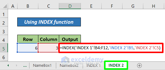
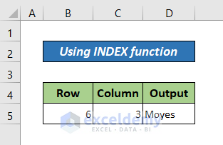
- Press Enter.
Note:
=INDEX(data range, row number, [column number])
Here,
- Data range is the entire table of the data
- Row number of the data is not necessarily the row of the Excel worksheet. If the table starts on row 5 of the worksheet, that will be Row #1.
- Column number of the data similarly depends on the Table. If the table range starts on column C, that will be column #1.
Download Practice Book
Download the following Excel file for your practice.
Related Articles
- Excel Formula to Get First 3 Characters from a Cell
- How to Extract Data from a List Using Excel Formula
- How to Extract Month and Day from Date in Excel
- How to Extract Month from Date in Excel
- How to Extract Year from Date in Excel
<< Go Back To Extract Data Excel | Learn Excel
Get FREE Advanced Excel Exercises with Solutions!
