7 Powerful Excel Functions That Aren’t VLOOKUP

 

Excel’s VLOOKUP function has been a go-to for many Excel users. But it comes with significant limitations: it can’t look left, it breaks when columns are moved, and it only returns the first match. Excel has several powerful alternatives that are more flexible and reliable.

In this tutorial, we will explore seven powerful Excel functions that aren’t VLOOKUP and can handle more complex scenarios with greater flexibility and efficiency.

Let’s consider a sample sales dataset to show how these powerful Excel functions can accomplish what VLOOKUP does—without using VLOOKUP.

1. XLOOKUP – The Modern VLOOKUP Replacement

XLOOKUP is Microsoft’s newest lookup function, designed to replace VLOOKUP entirely. It can search in any direction, return multiple values, and handle errors gracefully.

Syntax:

=XLOOKUP(lookup_value, lookup_array, return_array, [if_not_found], [match_mode], [search_mode])

Find Unit Price:

• Select a cell and insert the following formula

=XLOOKUP(A4, SalesData!E2:E51, SalesData!H2:H51,"Not found")

This formula can look left or right, doesn’t break if columns move, and handles missing keys gracefully. Available in Microsoft 365 and Excel 2021 or later.

Why Powerful:

• Searches left-to-right or right-to-left
• No need to count columns
• Has built-in [if_not_found] handling (no need for IFERROR)
• Supports exact, approximate, wildcard, and reverse lookups
• Can return multiple columns at once

2. HLOOKUP – Horizontal Lookup by Header

If your data is arranged in rows instead of columns, HLOOKUP works like VLOOKUP but horizontally.

Syntax:

=HLOOKUP(lookup_value, table_array, row_index_num, [range_lookup])

Lookup by Row:

• Select a cell and insert the following formula

=HLOOKUP(B3, SalesData!$A$1:$J$51, MATCH(A4, SalesData!$A$1:$A$51, 0), FALSE)

This formula is useful when datasets are stored in wide, row-based formats.

Why Powerful:

• Works when data is laid out horizontally instead of vertically
• An easy way to adapt if your dataset is structured in rows
• Familiar to VLOOKUP users but oriented differently

Note: HLOOKUP is now largely replaced by XLOOKUP, which works both vertically and horizontally.

3. INDEX & MATCH – The Flexible Powerhouse

This pairing combines INDEX (which returns a value at a specific position) with MATCH (which finds the position of a value). Together, they create a versatile lookup combination.

Syntax:

=INDEX(return_range, MATCH(lookup_value, lookup_array, 0))

Lookup Unit Price:

• Select a cell and insert the following formula

=INDEX(SalesData!H2:H51, MATCH(A4, SalesData!E2:E51, 0))

This formula extracts the unit price and functions similarly to XLOOKUP. You can use it in older versions of Excel.

Why Powerful:

• Works in any direction (left, right, up, down)
• Efficient with large datasets
• Doesn’t break when columns are inserted or deleted
• Can perform two-way lookups
• Available in older versions of Excel

4. FILTER – The Dynamic List Creator

The FILTER function returns multiple rows that meet specific criteria, creating dynamic lists that update automatically when source data changes.

Syntax:

=FILTER(array, include, [if_empty])

FILTER Sales (Multiple Criteria):

• Select a cell and insert the following formula

=FILTER(SalesData!A2:J51, (SalesData!D2:D51=A3) * (SalesData!I2:I51>100), "No matches")

This formula filters sales data based on region and a sales threshold. It is dynamic and automatically updates if any change occurs in the source data.

Why Powerful:

• Eliminates the need for manual filters or advanced formulas
• Can return multiple results at once, not just one
• Updates dynamically when new data is added
• Handles complex conditions easily
• Helpful for creating dynamic dashboards

5. SUMIFS & COUNTIFS – The Aggregation Masters

These functions perform lookups and simultaneously aggregate data based on multiple criteria.

SUMIFS Syntax:

=SUMIFS(sum_range, criteria_range1, criteria1, [criteria_range2, criteria2]...)

COUNTIFS Syntax:

=COUNTIFS(criteria_range1, criteria1, [criteria_range2, criteria2]...)

Total Sales by Region:

• Select a cell and insert the following formula

=SUMIFS(SalesData!$I$2:$I$51, SalesData!$C$2:$C$51, B4)

This formula looks up the East region, then sums the sales values to return the total sales for that region.

Total Orders per Region:

=COUNTIFS(SalesData!$C$2:$C$51, B4)

This formula counts the number of orders for each region.

Why Powerful:

• Performs lookup and aggregation in one formula
• Handles multiple conditions simultaneously
• Aggregates data instead of just returning values
• Faster than PivotTables for quick summaries
• Great for dashboards and KPI reporting

6. SORT/SORTBY, UNIQUE Function – Dynamic Functions

UNIQUE: Get Distinct Values

The UNIQUE function extracts distinct values from a list, helping build clean key lists for drop-downs and summaries.

Syntax:

=UNIQUE(array, [by_col], [exactly_once])

Distinct Items:

• Select a cell and insert the following formula

=UNIQUE(SalesData!E2:E51)

Returns the unique product list. This formula makes it easy to identify categories or remove duplicates without manual filtering.

Why Powerful:

• Instantly removes duplicates without extra steps
• Supports exactly_once mode (only values that appear once)
• Great for creating drop-down lists or distinct category lists
• Updates dynamically when new data is added

SORT / SORTBY: Sort by One or More Keys (even hidden ones)

The SORT/SORTBY functions organize your data dynamically without changing the original table—use them to present results cleanly or to prepare ranges for approximate matching.

Syntax:

=SORTBY(array, by_array1, sort_order1, [by_array2], [sort_order2], ...)

SORTBY Total and Data:

• Select a cell and insert the following formula

=SORTBY(SalesData!A2:J51, SalesData!I2:I51, -1, SalesData!B2:B51, 1)

This formula keeps the original dataset intact and allows easy sorting by multiple columns.

Why Powerful:

• Sorts an entire dataset based on another column
• Handles multiple sorting levels (e.g., by Date, then by Sales, etc.)
• Preserves all columns together while sorting (no broken rows)
• Automatically updates if source data changes

These pair perfectly with your lookups but aren’t lookups by themselves.

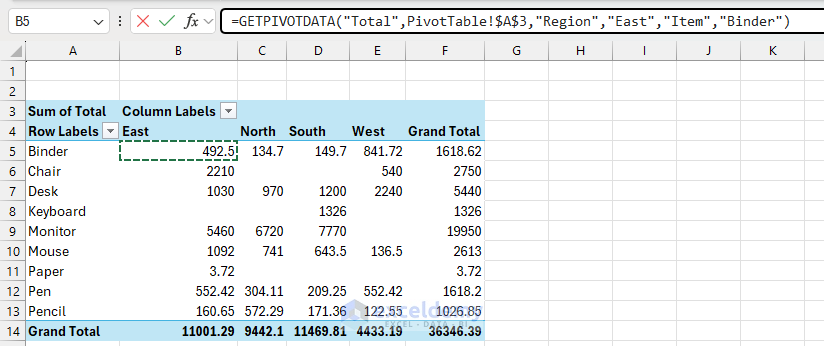
7. GETPIVOTDATA (PivotTable)

It is common to use PivotTables for data analysis. You can use GETPIVOTDATA to extract values directly without manual lookup.

Syntax:

=GETPIVOTDATA(data_field, pivot_table, [field1], [item1], …)

Sales for a Single Region:

• Select a cell and type equal (=)
• Go to the PivotTable sheet and select the cell

• Excel automatically creates the formula and returns the value

=GETPIVOTDATA("Total",PivotTable!$A$3,"Region","East","Item","Binder")

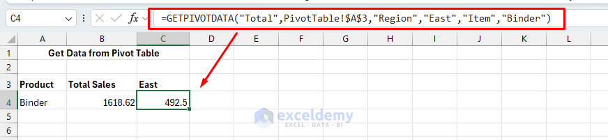
Ensures accurate lookups from PivotTables, unaffected by layout changes.

Why Powerful:

• Retrieves values from PivotTables accurately
• Works even if PivotTable layout changes
• Perfect for automated reports and dashboards

Pro Tips for Implementation

• Start Simple: Begin with XLOOKUP or INDEX/MATCH for basic VLOOKUP replacements
• Plan for Growth: Use functions that won’t break when data structure changes
• Combine Functions: Mix these functions for powerful solutions (e.g., INDEX/MATCH with FILTER)
• Test Thoroughly: Always test with edge cases and error conditions

Conclusion

These seven functions aren’t VLOOKUP but offer far more flexibility and power than VLOOKUP alone. By mastering them, you’ll be able to handle complex data scenarios that would be impossible or inefficient with traditional lookup methods. Based on your dataset and lookup type, choose the function that fits your current needs, then gradually incorporate others as you encounter more complex requirements.