Create a vacation calendar from 2021 to 2030 with a button to change the year.
Step 1 – Add a Spin Button to Select the Year
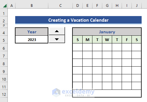
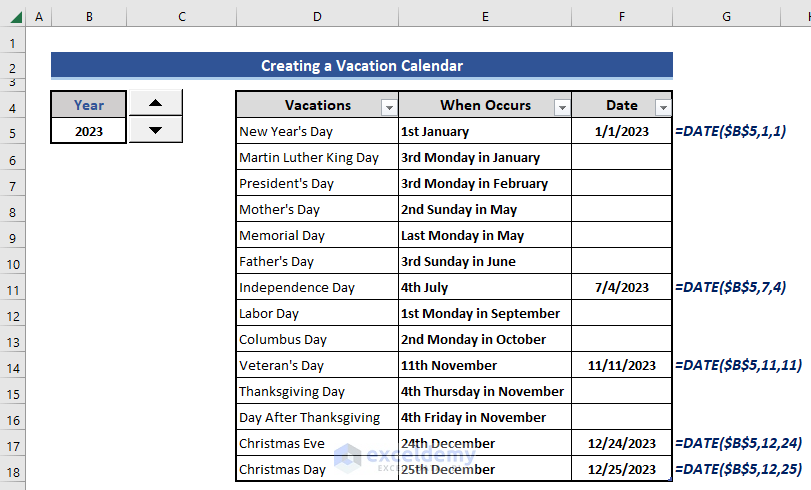
Look at the following image.
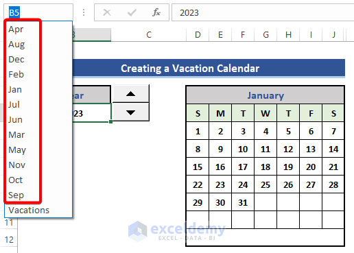
B5 contains the year.
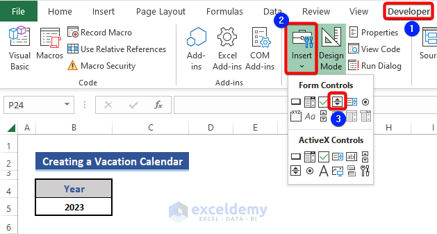
- Go to the Developer tab.
- Choose Insert in Control.
- Select Spin Button (Form Controls).
- Insert the Spin button in the dataset beside the Year cell.
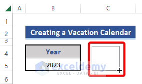
The Spin Button is displayed.

The up arrow will increase, and the down arrow will decrease the value.
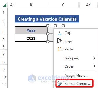
- Configure the Spin button.
- Select the Spin button and right-click.
- Choose Format Control.
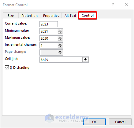
- In the Format Control window, choose Control.
- Enter values in Current value, Minimum value, Maximum value, and Incremental change.
- Select B5 as Cell link.
- Click OK.
You can change the year using the arrows.
Step 2 – Enter a Suitable Calendar Format
- Enter the name of the month and the first letter of the name of the day in the calendar format.
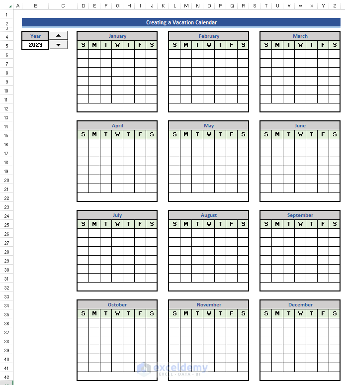
- Create the calendar format for the whole year.
Read More: How to Create Calendar with Time Slots in Excel
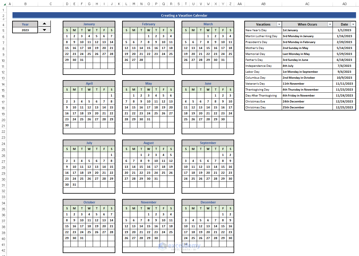
Step 3 – List All Holidays in the Year
- Enter the holidays in the calendar.
- Hide the calendar format.
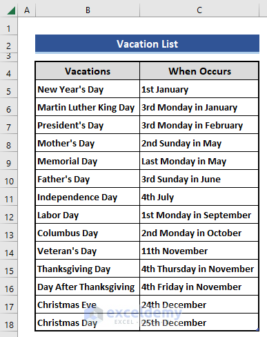
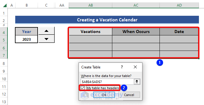
- Create a data table to enter the holidays with three columns: Vacation, When Occurs, and Date.
- Select the three columns and press Ctrl+T to create a table.
- In Create Table, check My table has headers and click OK.
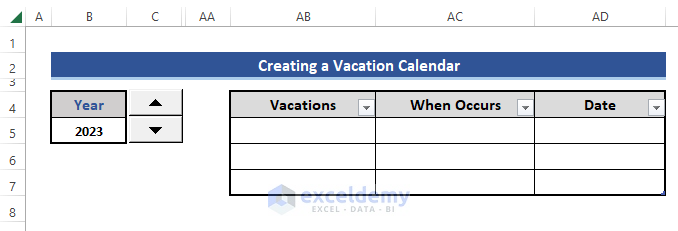
The Filter button is added to the dataset.
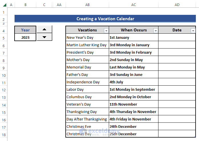
- Copy the data from the Vacation list and paste it into the dataset.
Formula to Enter Fixed Vacation Dates:
- Enter the formula in AD5.
=DATE($B$5,1,1)
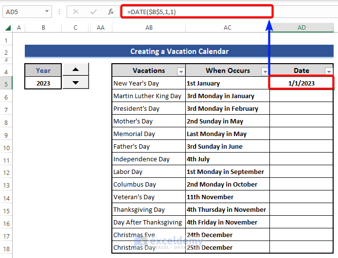
It returns: 1st of January.
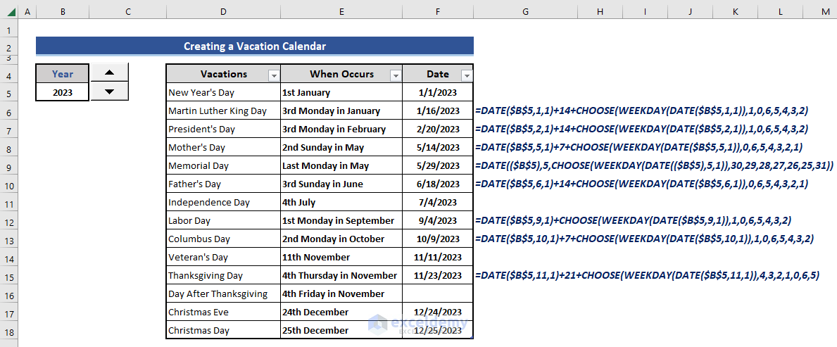
- Enter formulas for the rest of the fixed vacations.
Formula to Enter Variable Vacation Dates:
- Enter this formula in AD6.
=DATE($B$5,1,1)+14+CHOOSE(WEEKDAY(DATE($B$5,1,1)),1,0,6,5,4,3,2)
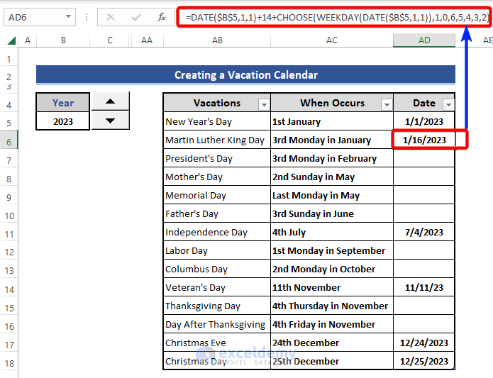
It returns data based on B5 that indicates the year.
- Use similar formulas for the rest of the moving vacation days.
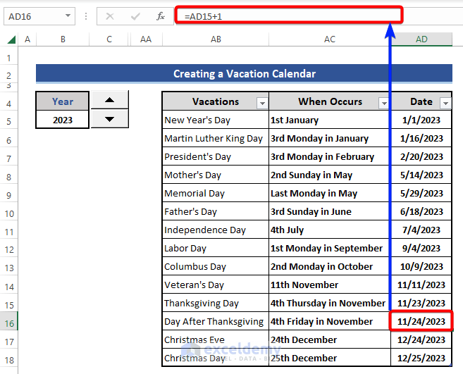
- There is a movable formula for AD16.
=AD5+1
Formula Explanation:
- DATE($B$5,1,1)
This returns a date value based on the input.
Result: 1/1/2023
- WEEKDAY(DATE($B$5,1,1))
This returns the respective number of weekdays from the applied date.
Result: 1/1/2023
- CHOOSE(WEEKDAY(DATE($B$5,1,1)),1,0,6,5,4,3,2)
The CHOOSE function will return a number based on the result of the WEEKDAY function. We used 1 for the second argument of the CHOOSE function to get Monday.
Result: 1
- =DATE($B$5,1,1)+14+CHOOSE(WEEKDAY(DATE($B$5,1,1)),1,0,6,5,4,3,2)
14 was added to get the 3rd Monday of the month with the previously calculated formulas.
Result: 1/16/2023
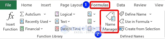
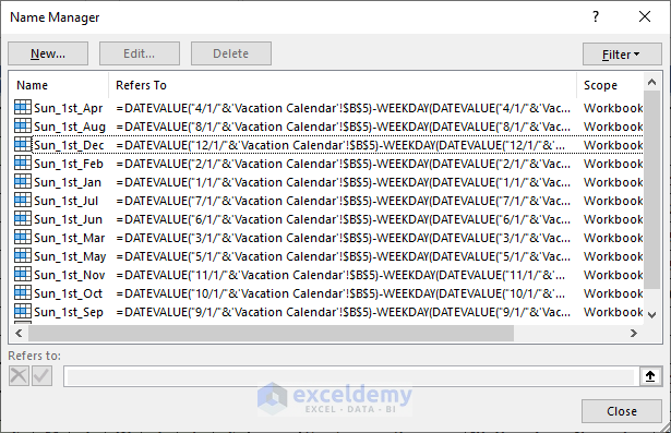
Step 4 – Define the Names of the Operational Factors
- Go to the Formulas tab.
- Click Name Manager in Defined Names.
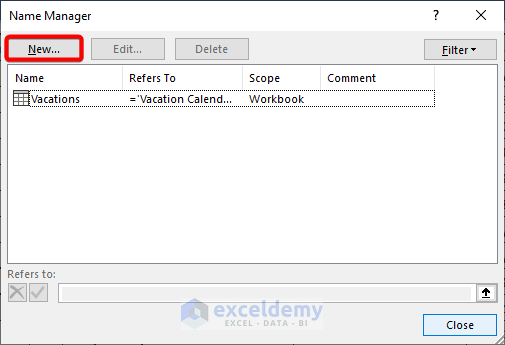
- In the Name Manager window, click New.
- In the New Name window, enter a name in Name.
- Enter the following formula in Refers to.
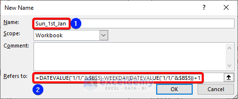
- Click OK.
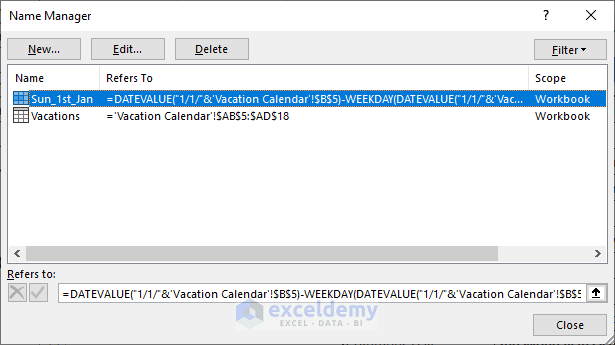
Name is added to the Name Manager. It will return the date of the 1st Sunday in the 1st week of January.
- Define new names for the 12 months, changing the date argument from “1/1/” to “2/1/” and so on. For December use:
=DATEVALUE("12/1/"&$B$5)-WEEKDAY(DATEVALUE("12/1/"&$B$5))+1
Step 5 – Enter a Formula to Insert Dates of Months in a Year
- Enter the formula in January.
- Go to D6 and use the following formula.
=IF(AND(YEAR(Sun_1st_Jan) = $B$5,MONTH(Sun_1st_Jan) = 1), Sun_1st_Jan, "")
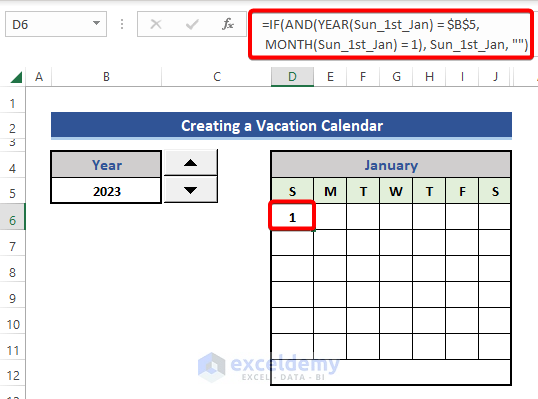
As the 1st day of January 2023 is Sunday, 1 is returned as the date.
- Go to E6 and enter this formula.
=IF(AND(YEAR(Sun_1st_Jan+1) = $B$5,MONTH(Sun_1st_Jan+1) = 1), Sun_1st_Jan+1, "")
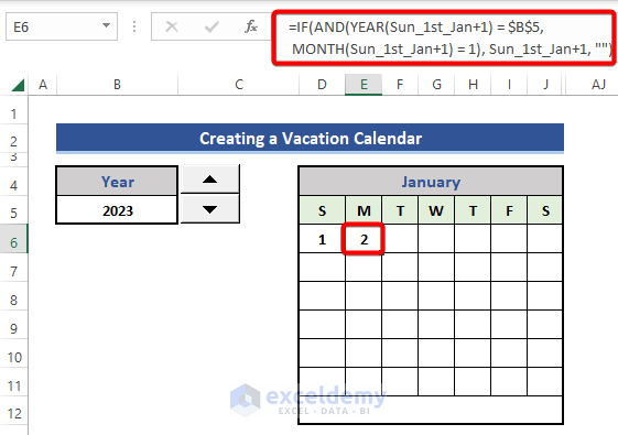
1 was added to Sun_1st_Jan. Use a similar formula and increase it 1 one by one for the rest of the cells.
- The formula used in J11 is:
=IF(AND(YEAR(Sun_1st_Jan+41) = $B$5,MONTH(Sun_1st_Jan+41) = 1), Sun_1st_Jan+41, "")
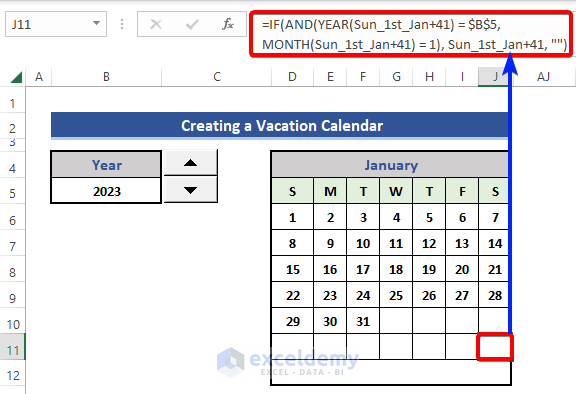
This is the last formula for January.
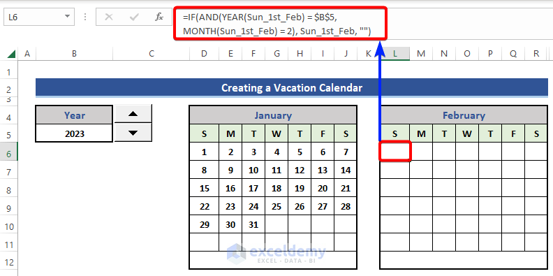
- For February, use this formula. Sun_1st_Jan was replaced with Sun_1st_Feb.
=IF(AND(YEAR(Sun_1st_Feb) = $B$5,MONTH(Sun_1st_Feb) = 2), Sun_1st_Feb, "")
- Input a similar formula to all cells for the other 11 months.
Formula Breakdown:
- YEAR(Sun_1st_Jan)
The YEAR function returns the year value of Sun_1st_Jan.
Result: 2023
- MONTH(Sun_1st_Jan)
The MONTH function returns the month value of Sun_1st_Jan.
Result: 1
- AND(YEAR(Sun_1st_Jan) = $B$5,MONTH(Sun_1st_Jan) = 1)
Checks if the year is equal to B5 and the month is equal to 1 for January.
Result: TRUE
- IF(AND(YEAR(Sun_1st_Jan) = $B$5,MONTH(Sun_1st_Jan) = 1), Sun_1st_Jan, “”)
If the condition is fulfilled, it returns the value Sun_1st_Jan, otherwise it returns blank.
Result: 1
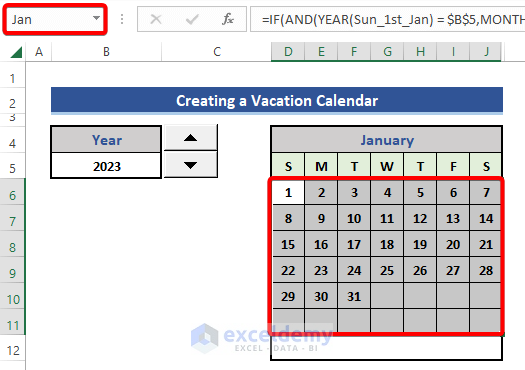
Step 6 – Define a Named Range for Each Month
- Select D6:J11.
- Go to the Name Box and enter Jan (short form for January).
- Enter the names of the rest of the months.
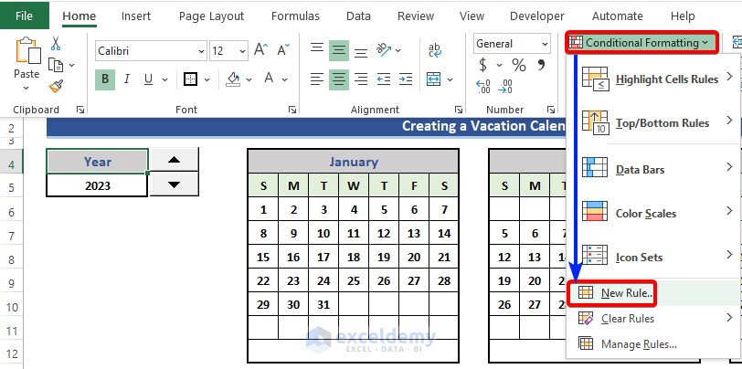
Step 7 – Apply Conditional Formatting to Highlight Vacations and Working Days
Highlighting Blank cells:
- Go to Conditional Formatting and choose New Rule.
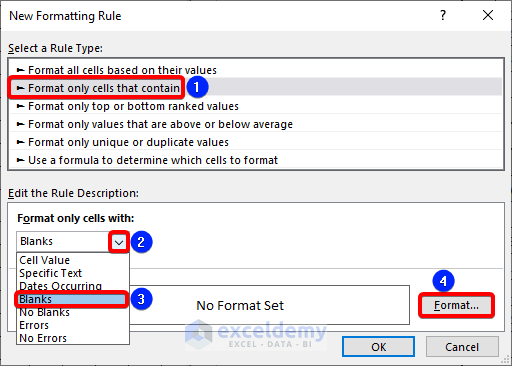
- Choose Format only cells that contain in Rule Type.
- Choose Blanks in Format only cells with.
- Click Format.
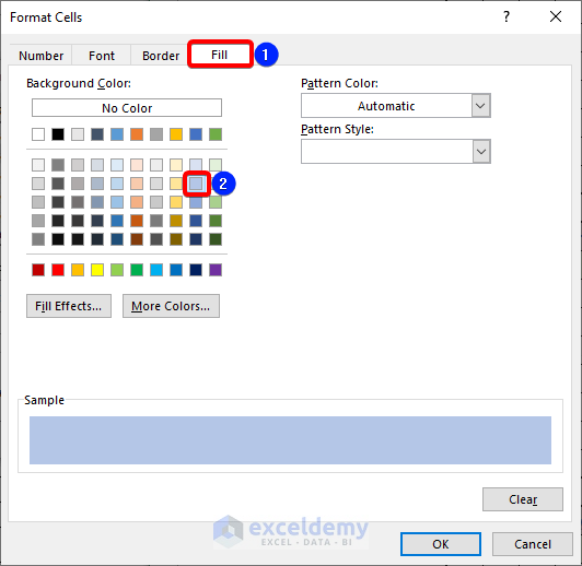
- Go to the Fill tab.
- Choose a color.
- Click OK.
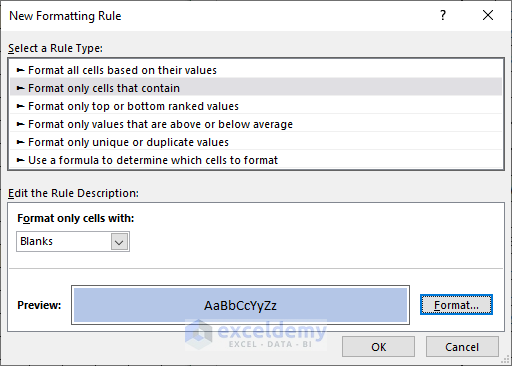
- Preview the selected format.
- Click OK.
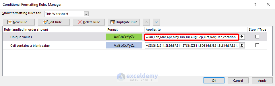
- To select a range to apply conditional formatting, go to Manage Rules in Conditional Formatting.
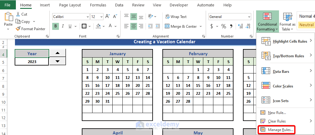
- In the Conditional Formatting Rules Manager window, go to Applies to and enter the following formula.
=Jan,Feb,Mar,Apr,May,Jun,Jul,Aug,Sep,Oct,Nov,Dec
- Click Apply and OK.
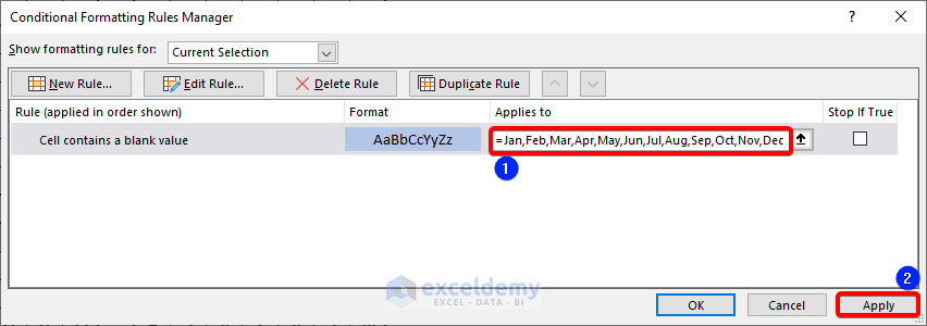
- Look at the calendar.
All blank cells are filled with the selected color.
Highlighting Working Days:
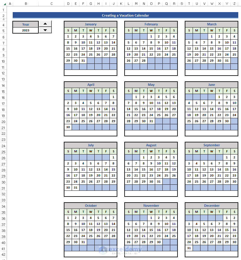
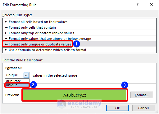
- Go to Conditional Formatting >> New Rules.
- Choose Format only unique or duplicate values.
- Choose Unique as the format.
- Select a color for the unique cells in Format.
- Go to Manage Rule and enter the range.
=Jan,Feb,Mar,Apr,May,Jun,Jul,Aug,Sep,Oct,Nov,Dec,Vacation
- Look at the calendar.
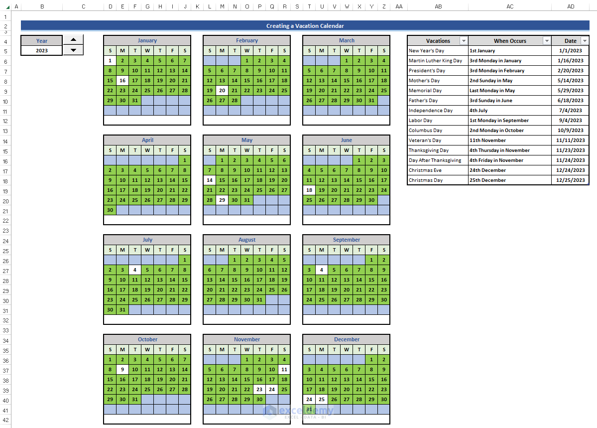
Vacation days contain the default color.
Step 8 (Optional) – Calculate Total Vacations
- Go to D12 and enter the following formula.
="Total Vacations: "&SUMPRODUCT(COUNTIF(Jan,Vacation))
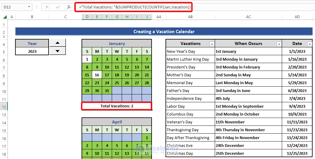
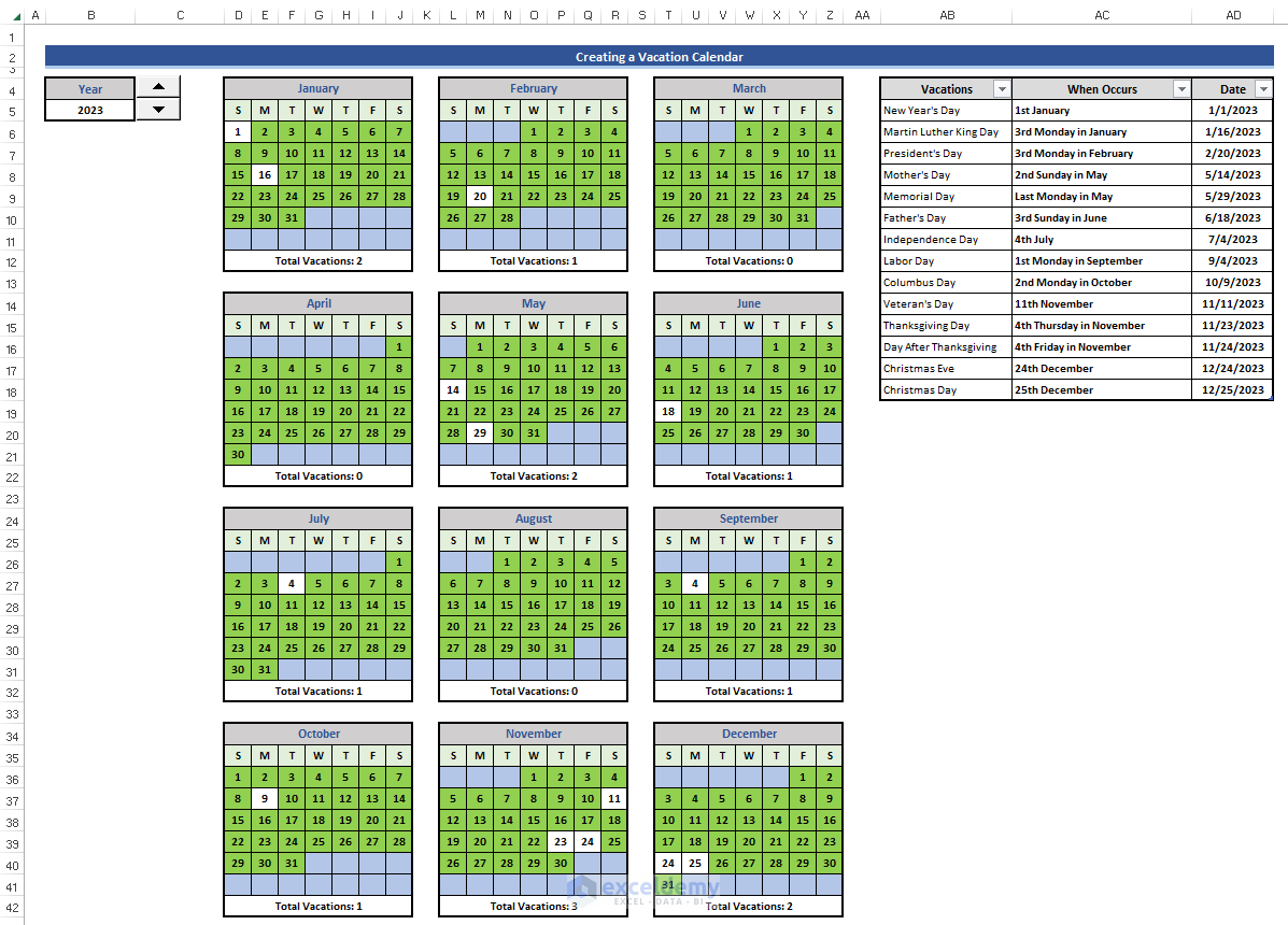
The total vacation days in January will be displayed.
- Use similar formulas for the other 11 months, changing the name of the months.
Download Practice Workbook
Download the practice workbook to exercise.
Related Articles
<< Go Back to Excel Calendar Templates | Excel Templates
Get FREE Advanced Excel Exercises with Solutions!
