
Manipulating dates to extract specific components like month, quarter, and year: these date format transformations are essential for data analysis, making it easier to group data by year and month. In this article, we will show how to transform date format to month, quarter, and year in Excel using practical examples.
1. Extracting the Month from a Date
To transform a date into a month or to extract the month from a date, you can use the MONTH and TEXT functions, which return the month number and full month name.
Use the MONTH Function
The MONTH function returns the month as a number (1 for January, 2 for February, etc.). Insert the following formula in the B2 cell.
Formula:
=MONTH(A2)
This returns the month number of the date of the A2 cell.
Output:

Use the TEXT Function to Get the Month’s Name
You can display the full or abbreviated month name by using the TEXT function.
To get the full month name, insert the following formula in cell C2.
Formula:
=TEXT(A2, "MMMM")
The TEXT function will return the full month name for the A2 cell following the format code “MMMM”. This will return “January” for dates in January, “February” for February, and so on.
Output:

To get the abbreviated month, insert the following formula in cell D2.
Formula:
=TEXT(A2, "MMM")
This formula will return a three-letter abbreviation of the month following the format code “MMM”.
Output:

2. Extracting the Quarter from a Date
You can calculate the quarter from a date by using Excel formulas. Since Excel doesn’t have a built-in function for quarters, you can use a combination of formulas. Insert the following formula in cell E2.
Formula:
=ROUNDUP(MONTH(A2)/3, 0)
This formula divides the month by 3 (since there are three months per quarter) and rounds up to the next whole number.
- Months 1-3 as Q1
- Months 4-6 as Q2
- Months 7-9 as Q3
- Months 10-12 as Q4
Output:

Display the Quarter with Text (e.g., “Q1”, “Q2”):
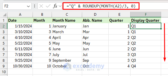
To get a descriptive format, you can add text like “Q1,” “Q2,” etc. in Excel. Use the & operator to concatenate “Q” with the quarter number. Insert the following formula in cell F2.
Formula:
="Q" & ROUNDUP(MONTH(A2)/3, 0)
This formula will concatenate the Q with the Quarter number of the date. As A2 contains 1/15/2024, the formula will return Q1.
Output:
3. Extracting the Year from a Date
You can use the YEAR function to retrieve the year from a date. Insert the following formula in cell G2.
Formula:
=YEAR(A2)
This formula will return the year from the date of the A2 cell. This function is especially useful for aggregating data by year.
Output:

4. Combining Year and Quarter
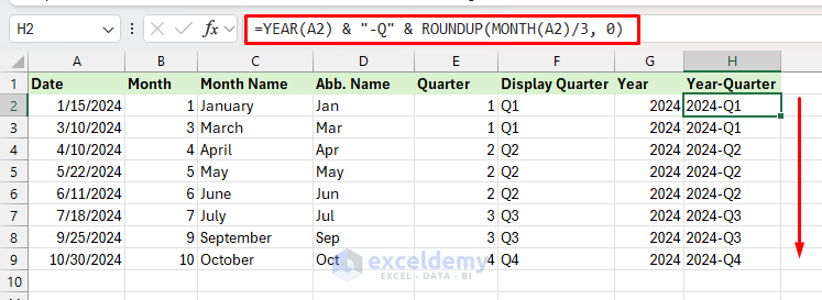
You can create a year-quarter label (like “2024-Q1”) by combining the YEAR ROUNDUP and MONTH functions. Insert the following formula in cell H2.
Formula:
=YEAR(A2) & "-Q" & ROUNDUP(MONTH(A2)/3, 0)
This formula combines the year and quarter to create a unique label for each quarter within a year. This formula helps to track data by fiscal quarter within a specific year.
Output:
5. Formatting Dates Using Custom Date Formats
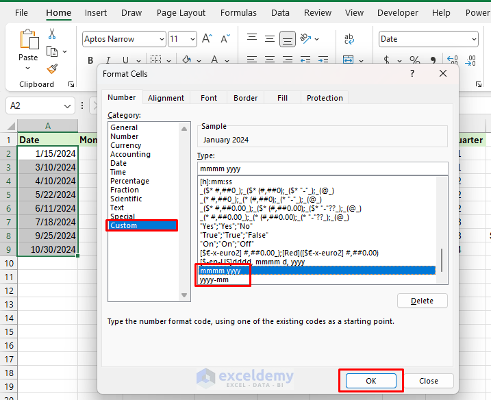
You may only want to change how the date looks without altering the actual date value, Excel’s custom formatting can further adjust how dates appear, without changing the underlying data.
- Select the cells containing dates.
- Press Ctrl+1 to bring the Format Cells dialog box >> select Custom.
- To display only the month and year (e.g., “January 2024”).
"MMMM YYYY"
- To display year and month in ISO format (e.g., “2024-1”).
"YYYY-MM"
Conclusion
You can transform your date formats by following the formulas and formatting options. Excel formulas help to manipulate dates, transforming them into month, quarter, and year-based representations to enhance your data analysis capabilities. Explore all the formatting options and functions to manipulate the dates.
Get FREE Advanced Excel Exercises with Solutions!
