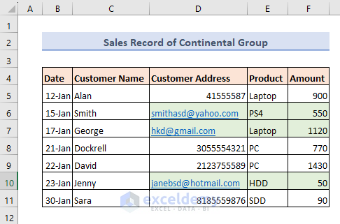
The following dataset contains sales records of the Continental Group for January. It includes information such as the date of the sale, the name and contact information of the customer, the product sold, and the amount of the sale. The products sold in this dataset are laptops, PS4s, PCs, HDDs, and SDDs. Let’s add cells based on various criteria using the textual values in the dataset.
Method 1 – Sum If Cell Contains Text
We will add the quantities of products whose customers’ addresses are Email IDs rather than Phone Numbers.
Case 1.1 – Using the SUMIF Function to Sum if a Cell Contains Text in Excel
Excel’s SUMIF function can be used to sum if a cell contains the text.
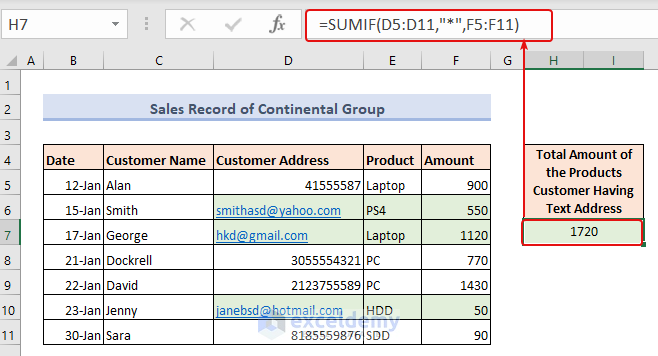
- Use an Asterisk Symbol (*) as the condition in a SUMIF function, as seen in the formula below:
=SUMIF(D5:D11,"*",F5:F11)Case 1.2 – Combine SUM, IF, and ISTEXT Functions to Sum If a Cell Contains Text in Excel
- Select any cell on the worksheet and then enter the following formula:
=SUM(IF(ISTEXT(D5:D11),F5:F11,0))We’ve got the same total amount of products with customers having text addresses, 1720.
Note: It’s an array formula, So if you aren’t a Microsoft 365 user, use CTRL+SHIFT+ENTER.
Formula Breakdown:
ISTEXT(D5:D11) checks each value in the range D5:D11 and returns a TRUE if it’s a text value. Otherwise, it returns a FALSE.
It returns the corresponding value from the range F4:F11 for each TRUE. And for each FALSE, it returns 0.
Therefore the formula becomes SUM(0,F6,F7,0,0,F10,0).
Now the SUM function returns the sum of the corresponding values from the range F4:F11.
Case 1.3 – Utilizing the SUMIF Function to Sum by Using Cell Number
By using a cell number, we can find specific text in the dataset and sum the value according to our criteria.
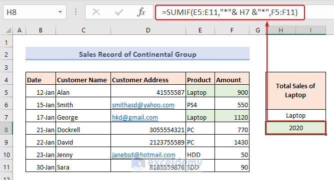
- Select cell number H8 and enter the following formula:
=SUMIF(E5:E11,"*"& H7 &"*",F5:F11)
The total amount of Laptops is 2020.
Short Explanation of the Formula:
The SUMIF function will look for the text value of cell H7.
So, the SUMIF function searches for “Laptop” in the cells E5:E11. It returns True if “Laptop” is found. Otherwise “False”
Now the SUMIF function returns the sum of the corresponding values from the range F4:F11.
Case 1.4 – Use Excel’s SUMIF Function (Case-Insensitive Match)
We’ll add up the cells that have text values with a certain text. We’ll sum any cell that contains the text “pc” in it.
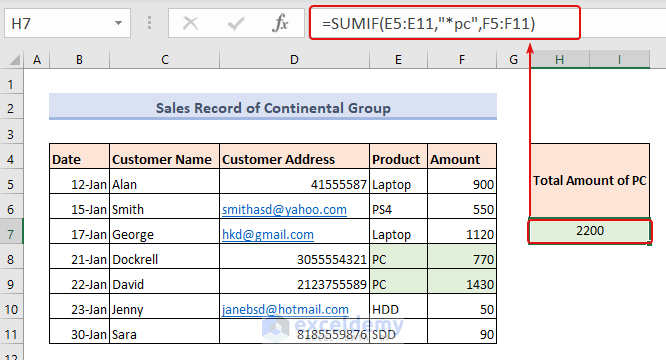
- Enter the following formula in any cell of your datasheet:
=SUMIF(E5:E11,"*pc",F5:F11)
The total amount of “pc” product is 2200.
Case 1.5 – Use SUMPRODUCT, ISNUMBER, and FIND Functions (Case-Sensitive Match)
We will apply a formula combination of SUMPRODUCT, ISNUMBER, and FIND functions for a case-sensitive match.
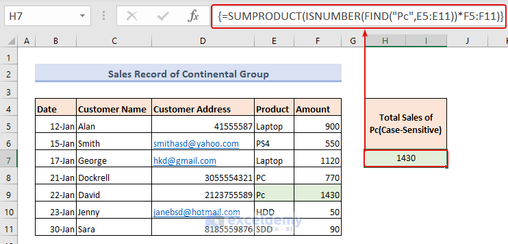
- Use the following formula to find items that have exactly “Pc” in the Product name:
=SUMPRODUCT(ISNUMBER(FIND("Pc",E5:E11))*F5:F11)
The outcome is 1430. There is only one cell containing the text “Pc”
Note: It’s an Array Formula. So press CTRL+SHIFT+ENTER unless you are using Microsoft Office 365.
Read More: How to Use Excel SUMIF with Greater Than Criterion
Case 1.6 – Applying the SUMIFS Function to Sum If a Cell Contains Text in Excel
To sum if a cell contains text, we can use the SUMIFS function rather than the SUMIF function in Excel.
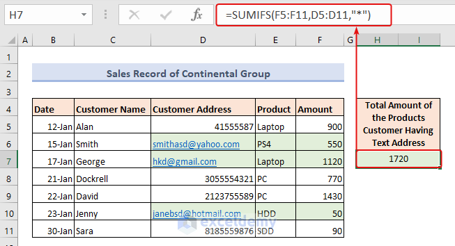
- Use the following formula:
=SUMIFS(F5:F11,D5:D11,"*").The total amount of products customers have text addresses is 1720.
Formula Breakdown:
The SUMIFS function takes a sum_range and one or more pairs of range and criteria.
Here our sum_range is F5:F11 (Amounts). And we have used one pair of a range and criteria.
The range is D5:D11 (Contact Address), and the criteria is “*”. It searches for all the text values within the range D5:D11.
When it finds a text value in the range D5:D11, it sums the corresponding value from the sum_range F5:F11
Thus SUMIFS(F5:F11,D5:D11,”*”) returns the sum of all the amounts from the range F5:F11where the corresponding address in the range D5:D11 is a text address.
Method 2 – Sum Cells Containing Numbers Only
Case 2.1 – Using a Combination of SUM, IF, and ISNUMBER Functions to Sum if a Cell Contains a Number
We can use SUM, IF, and ISNUMBER functions to sum up if a cell contains a number in Excel.
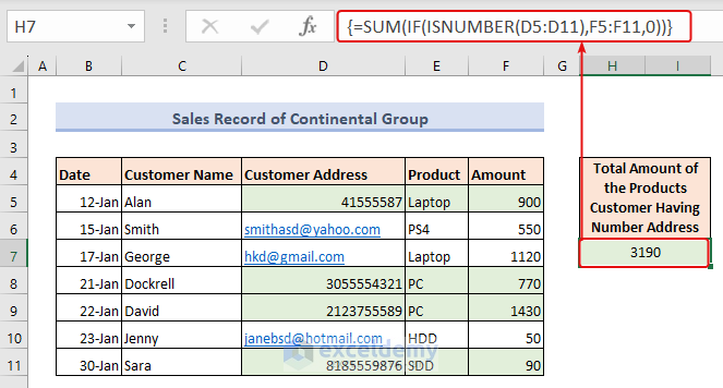
- Select a cell on the worksheet and Enter the formula below:
=SUM(IF(ISNUMBER(D5:D11),F5:F11,0))Formula Breakdown:
- ISNUMBER(D5:D11) returns an array of TRUE or FALSE values, indicating whether each cell in the range D5:D11 contains a number or not.
- IF(ISNUMBER(D5:D11),F5:F11,0) returns an array of values, where each value is either the value in the corresponding cell in the F range (if the corresponding cell in the D range contains a number), or 0 (if the corresponding cell in the D range does not contain a number).
- SUM(IF(ISNUMBER(D5:D11),F5:F11,0)) calculates the sum of the array returned in step 2, which gives us the total sum of the values in the F range for cells where the corresponding cell in the D range contains a number.
Method 3 – Sum Cell Containing Both Texts and Numbers
We’ll change the dataset slightly to include storage capacities, which are in GBs and TBs. We are going to calculate the total storage capacity based on the type of storage.
We also added GB(Gigabyte) and TB(Terabyte) in cells H7 and H8.
Case 3.1 – Combining Several Excel Functions to Sum if a Cell Contains Both Text and Numbers in Excel
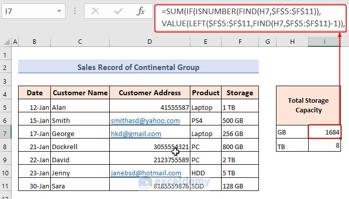
- Select any cell on your dataset. Here we took I7.
- Enter the formula below:
=SUM(IF(ISNUMBER(FIND(H7,$F$5:$F$11)),VALUE(LEFT($F$5:$F$11,FIND(H7,$F$5:$F$11)-1)),0))The total Storage capacity is 1684GB and 8TB
Note: This is an array formula. Press Ctrl + Shift + Enter to apply it unless you are using Microsoft Office 365
Formula Breakdown:
FIND(H7,$F$5:$F$11) returns an array of the position of the substring H7 in each cell in the range $F$5:$F$11. If the substring is not found, it returns an error.
ISNUMBER(FIND(H7,$F$5:$F$11)) converts the array from step 1 into an array of TRUE or FALSE values, where TRUE indicates that the substring is found in the corresponding cell and FALSE indicates that it is not found.
LEFT($F$5:$F$11,FIND(H7,$F$5:$F$11)-1) returns an array of the leftmost characters in each cell in the range $F$5:$F$11 up to the position of the substring H7. If the substring is not found, it returns an error.
VALUE(LEFT($F$5:$F$11,FIND(H7,$F$5:$F$11)-1)) converts the array from step 3 into an array of numerical values.
IF(ISNUMBER(FIND(H7,$F$5:$F$11)),VALUE(LEFT($F$5:$F$11,FIND(H7,$F$5:$F$11)-1)),0) returns an array of numerical values or 0, depending on whether the substring is found in each cell in the range $F$5:$F$11 or not.
SUM(IF(ISNUMBER(FIND(H7,$F$5:$F$11)),VALUE(LEFT($F$5:$F$11,FIND(H7,$F$5:$F$11)-1)),0)) calculates the sum of the array returned in step 5, which gives us the total sum of the numerical values extracted from cells that contain the substring H7.
Method 4 – Sum Numbers in a Cell with a User-Defined Function That Ignores Text
We want to sum only the numerical values strings which contain both text and numerical values.

- Press Alt + F11 to open the Microsoft Visual Basic for Applications window.
- Click Insert and select Module.
- Paste the following code in the Module Window.
Code:
Function SumNumbers(rngS As Range, Optional strDelim As String = " ") As Double
'Update by Exceldemy
    Dim NUM As Variant, Total As Long
    NUM = Split(rngS, strDelim)
    For Total = LBound(NUM) To UBound(NUM) Step 1
        SumNumbers = SumNumbers + Val(NUM(Total))
    Next Total
End Function- Save and close the code and go back to the worksheet.
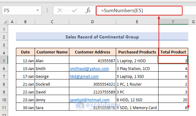
- Enter the below formula on your worksheet,
=Sumnumbers(E5)- Drag the fill handle down to the cells you want to fill the formula, and only numbers in each cell are added together, see the picture above.
Here E5 indicates the cell where you only want to sum up the numbers.
Frequently Asked Questions
How do I sum cells with text and numbers in Excel?
To sum cells with text and numbers in Excel, you can use the SUMIF function. Here’s how you do it:
- Choose a cell where you want to see the sum.
- Type “=SUMIF(range, criteria, sum_range)” in the cell.
- In the “range” section, select the cells you want to sum up.
- At the “criteria” section, type the text and number you want to sum up.
- In the “sum_range” section, select the cells you want to sum up that match the criteria.
- Press “Enter” to see the sum of the cells that contain the text and number you entered.
If the cells have both text and numbers, you may need to use other functions like LEFT, RIGHT, and SUM to separate and add the numbers and text separately.
How do I add to the sum if a cell contains text in Excel?
To add to the sum of cells that contain text in Excel, you can use the SUMIF function with wildcards.
For example, if you want to add up the values in cells that contain the word “orange“, you would enter “=SUMIF(A1:A10, “orange”, B1:B10)” in the cell where you want to see the sum. This formula would add up the values in cells B1 to B10 where the corresponding cells in A1 to A10 contain the word “orange“, no matter what other characters are before or after it.
Remember that the SUMIF function is not case-sensitive, so it will match text regardless of whether it is in uppercase or lowercase.
3. How do I combine text and numbers in two cells in Excel?
To combine text and numbers in two cells in Excel, you can use the CONCATENATE function.
For example, if you want to combine the text “Order #” in cell A1 with the number “123” in cell B1, you would enter “=CONCATENATE(A1, B1)” in the cell where you want to see the combined result. This formula would give you “Order #123“.
Download the Practice Workbook
Related Articles
- How to Use Excel SUMIF to Sum Values Greater Than 0
- How to Use SUMIF to SUM Less Than 0 in Excel
- Sum If Greater Than and Less Than Cell Value in Excel
- How to Use 3D SUMIF for Multiple Worksheets in Excel
- How to Use Excel SUMIF Function Based on Cell Color
<< Go Back to Excel SUMIF Function | Excel Functions | Learn Excel
Get FREE Advanced Excel Exercises with Solutions!
