We will use a sample dataset where the sales of computers of different brands have been recorded over 6 months.

Method 1 – Using the SUMPRODUCT Function to Sum Based on Column and Row Criteria
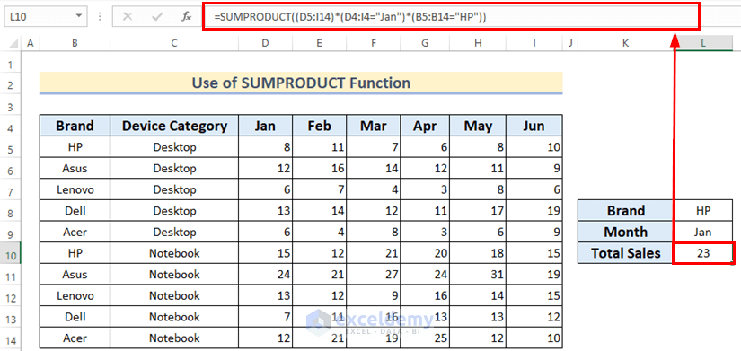
We’ll find the number of HP devices sold in January.
Steps:
- Cells L8 and L9 contain the conditions.
- Insert the following formula in cell L10.
=SUMPRODUCT((D5:I14)*(D4:I4="Jan")*(B5:B14="HP"))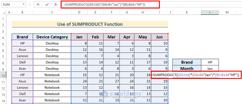
- Hit Enter to get the result.
Read More: How to Apply SUMIF with Multiple Ranges in Excel
Method 2 – Combining SUM and IF Functions to Sum under Column and Row Criteria
Steps:
- Cells L8 and L9 contain the conditions.
- Insert the following formula in cell L10.
=SUM(IF(D4:I4=L9,IF(B5:B14=L8,D5:D14)))- Press Enter.
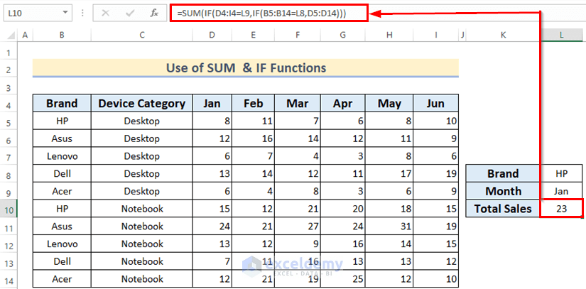
How Does This Formula Work?
- By combining two IF functions in the arguments, the formula goes through all the sales recorded in the chart & returns as {8,15, FALSE, FALSE…}.
- The SUM function then sums up the number values to 23 (8+15).
Method 3 – Applying SUMIF Function to Sum Based on Column and Row Criteria
Case 1 – Using SUMIF with Multiple AND Criteria
Steps:
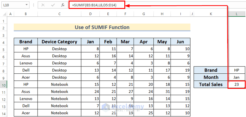
- Cells L8 and L9 contain the conditions.
- Insert the following formula in cell L10.
=SUMIF(B5:B14,L8,D5:D14)- Press Enter.
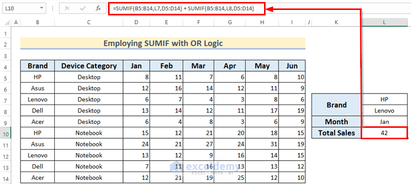
Case 2 – Using SUMIF with Multiple OR Criteria
We’ll find out the number of HP as well as Lenovo devices sold in January.
Steps:
- Cells L7 and L8 contain the OR conditions, while L9 contains the month.
- Insert the following formula in cell L10.
=SUMIF(B5:B14,L7,D5:D14) + SUMIF(B5:B14,L8,D5:D14)The formula manually goes through the Jan column via the D5:D14 argument.
- Hit Enter.
Read More: How to SUMIF for Multiple Criteria Across Different Sheet in Excel
Method 4 – Incorporating SUMIF, INDEX, and MATCH Functions in Excel
Steps:
- Cells L8 and L9 contain the conditions.
- Insert the following formula in cell L10.
=SUMIF(B5:B14,L8,INDEX(D5:I5,MATCH(L9,D4:I4,0)))- Hit Enter.
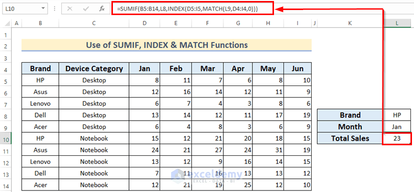
How Does This Formula Work?
- The MATCH function looks for the position of the month Jan in the range of cells D4:I4.
- The INDEX function stores all the sales in the column of Jan as a reference.
- The SUMIF function finally sums up the sales of HP devices only.
Method 5 – Using the SUMIFS Function to Sum Based on Column and Row Criteria
SUMIFS is the subcategory of the SUMIF function which implicitly sums the range of cells if all the corresponding cells fulfill their respective criteria. It has a slightly different syntax:
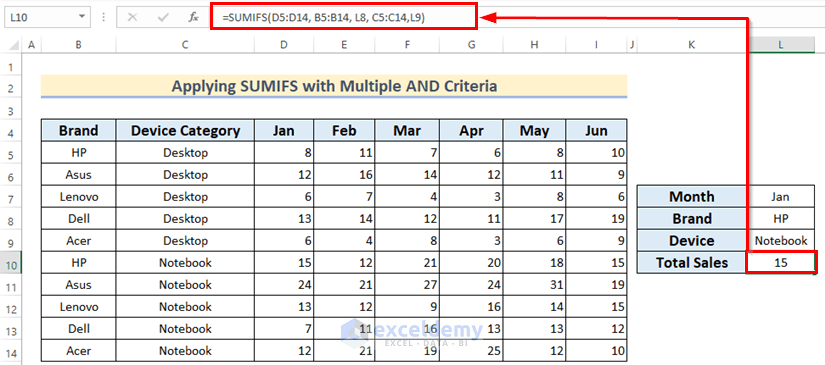
Case 1 – Using SUMIFS to SUM under Multiple AND Criteria Based on Column and Row
Steps:
- Cells L7 and L8 contain the AND conditions.
- Insert the following formula in cell L10.
=SUMIFS(D5:D14, B5:B14, L8, C5:C14,L9)- Hit Enter.
Read More: SUMIF with Multiple Criteria in Different Columns in Excel
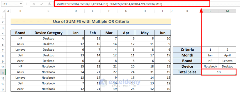
Case 2 – Use SUMIFS with Multiple OR Criteria to Sum Based on Data Columns and Rows
We want to know the total number of sales of HP notebooks in January and Lenovo desktops in April.
Steps:
- The range L8:M10 contains the conditions.
- Insert the following formula in cell L11.
=SUMIFS(D5:D14,B5:B14,L9,C5:C14,L10)+SUMIFS(G5:G14,B5:B14,M9,C5:C14,M10)- Hit Enter.
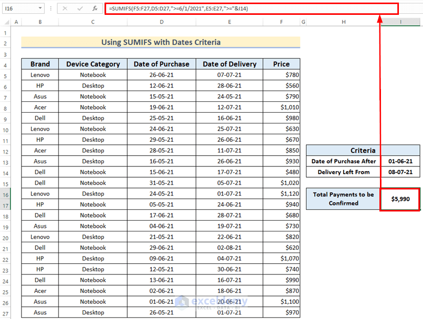
Case 3 – Using SUMIFS to Sum Based on Column and Row Criteria with Dates
We have the dates of purchase, dates of delivery and the prices of the devices for various sales. We want to know the total payments that the shop will receive after delivering the rest of the products (purchased after May) from the date 08-July-2021.
Steps:
- In cell I16, insert:
=SUMIFS(F5:F27,D5:D27,">=6/1/2021",E5:E27,">="&I14)- Hit Enter.
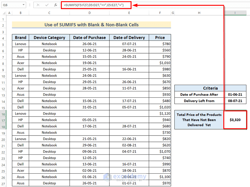
Case 4 – Inserting SUMIFS to Sum under Column and Row Criteria with Blank and Non-Blank Cells
There are a few missing values in the columns of Date of Purchase & Date of Delivery. We want to know the total price of the products that have been purchased but not delivered yet.
Steps:
- In cell I16, our formula for the given criteria will be:
=SUMIFS(F5:F27,D5:D27,"<>",E5:E27,"=")- Hit Enter.
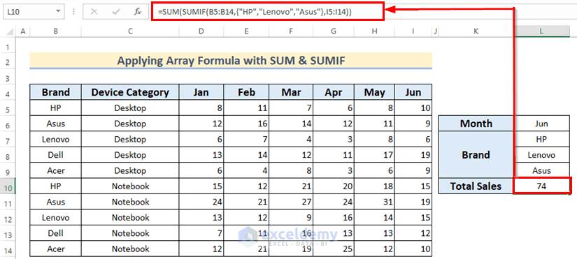
Method 6 – Using an Array Formula to Sum Based on Column and Row Criteria
We’ll determine the total number of sales in June for HP, Lenovo, and Asus devices.
Steps:
- In cell L10, insert:
=SUM(SUMIF(B5:B14,{"HP","Lenovo","Asus"},I5:I14))- Press Enter.
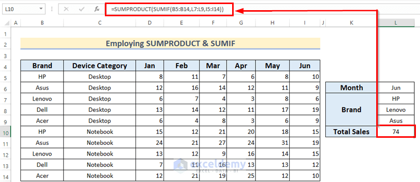
Method 7 – Using SUMPRODUCT and SUMIF Functions Together to Sum under Column and Row Criteria
Steps:
- In cell L10, the formula will be:
=SUMPRODUCT(SUMIF(B5:B14,L7:L9,I5:I14))- Hit Enter.
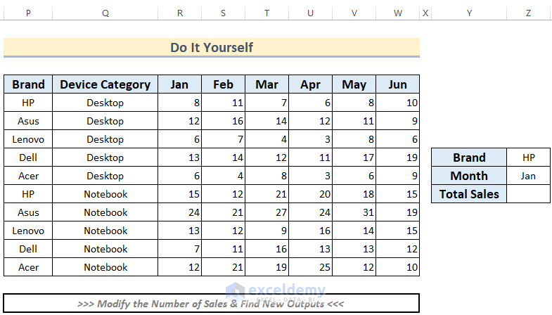
Practice Section
You can practice the explained methods by yourself in the download file.
Download the Practice Workbook
Related Articles
<< Go Back to SUMIF Multiple Criteria | Excel SUMIF Function | Excel Functions | Learn Excel
Get FREE Advanced Excel Exercises with Solutions!
