In this article, we will learn to use smart tags in Excel. Assume we have a dataset and now we want to add new information by adding rows or columns. We can easily do that by using smart tags. Not only that, but we can also identify errors, analyze data, flash-fill the cells automatically, and many more. Today, we will show 7 important and widely used applications of smart tags. So, without any delay, let’s start the discussion.
What Are Smart Tags in Excel?
Smart Tag is a small button that occurs during selecting a cell or working with data in the cell and can easily access the work with just a single click. We can enable and disable the smart tags as per our demands.
How to Enable/Disable Smart Tags in Excel
To enable the smart tag, we need to do some preceding according to the smart tag we want to put in our system. And for disabling the smart tag, we need to undo the process. This process of enabling or disabling depends on what type of smart tag you are working on. We will describe the enable and disable processes of different smart tags with the following examples.
How to Use Different Smart Tags in Excel: 7 Examples
There are various types of smart tags available. Here we will work with the most popular 7 examples of smart tags that we use every day to save time and do the work more efficiently.
1. Utilize AutoCorrect Smart Tag to Make Automatic Correction in Excel
AutoCorrect smart tag is very popular and mainly used for our written mistakes. Sometimes we write the wrong word by mistake, and with the AutoCorrect smart tag, we can easily correct the mistakes. Let’s follow the method to learn the procedure.
STEPS:
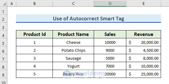
- First of all, you need to make the dataset ready.
- To do so, insert the data in an Excel sheet.
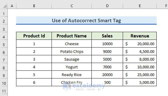
- Here, we have used the range B4:E9 to insert the sales information.
- Secondly, from the ribbon, we have to select the File tab.
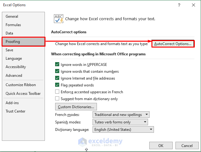
- Now, a new window will open up and from the leftmost corner select Options.

- After that, Excel Options window will appear on the screen.
- Now, from the Proofing section, we have to click AutoCorrect Options.
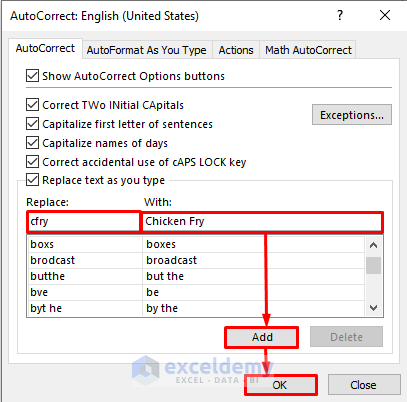
- In the AutoCorrect menu box, check all options.

- After checking, we will insert our input and output.
- We want that if you write cfry, Excel will automatically detect that we are talking about Chicken Fry.
- Therefore, we will put cfry in Replace column and Chicken Fry in With column.
- You can change your input and output as per your expectations.
- In our dataset, we will add another type of data.
- We will input cfry as Product Name as press ENTER.

- As a result, cfry is automatically replaced by Chicken Fry.
- After that, fill in the information.
- You may spell the word incorrectly.
- Instead of Chilli Chips we may insert chillli chipps.
- If we knew before, we can replace chillli chipps with Chilli Chips which is the correct one.

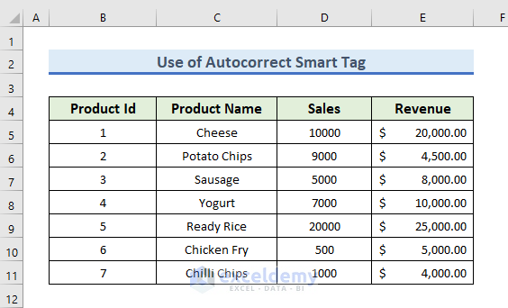
- Now, we will insert Chilli Chips information.
- By mistake we have written chillli chipps.

- Excel will correct the information to Chilli Chips.
- Now fill in the other information.
Read More: How to Add Tags in Excel
2. Use Paste Smart Tag to Paste Data in Excel
Paste smart tag is a very useful tag as we can copy and paste as per our expectations. We can paste with and without formatting. Also, various types of pasting methods are available here. Let’s follow the method to learn the procedure.
STEPS:
- First of all, you need to make the dataset ready.
- To do so, insert the data in an Excel sheet.
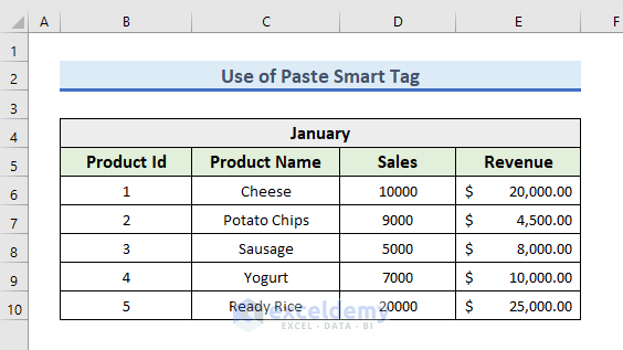
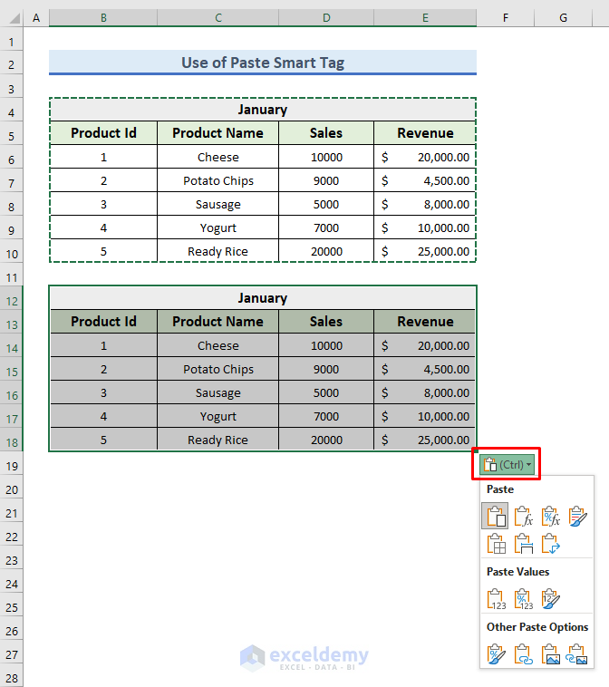
- Here, we have used the range B5:E10 to insert the sales information for January month.
- Firstly, select File from the ribbon.

- Secondly, a new window will open up, and from the leftmost corner select Options.

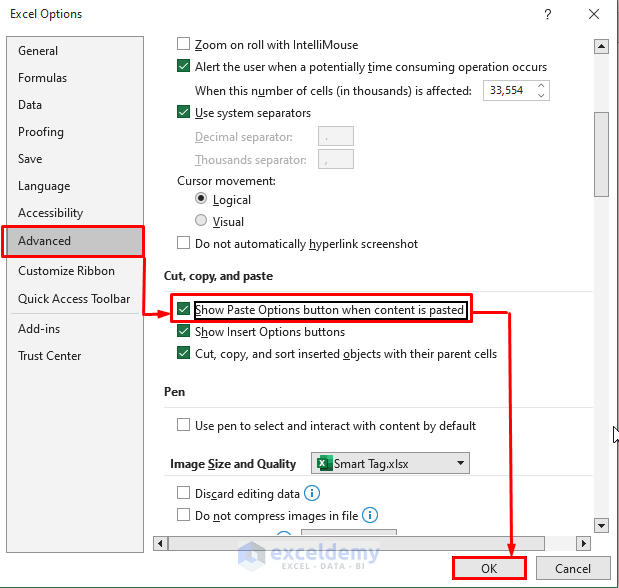
- From the Excel Options window, find the Advanced option.
- In the Advanced option, check Show Paste Options button when content is pasted and press OK.
- We want to make another dataset of February month from this dataset.
- So, select the entire dataset.

- Press Ctrl + C to copy the dataset.
- After that, select Cell B12 and press Ctrl + V to paste it.
- We are seeing a smart tag of paste near the end of the dataset.
- Click on the smart tag and you can modify the paste as per your wish.
- For disabling the Paste smart tag, uncheck Show Paste Options button when content is pasted in the Excel Options box.

Read More: How to Make Name Tags in Excel
3. Employ AutoFill Smart Tag to Fill Cells in Excel
By using the AutoFill smart tag, Excel can identify if you are trying to rewrite the same information written before, and with just one click, you can AutoFill the information if it is correct.
STEPS:
- First of all, you need to make the dataset ready.
- To do so, insert the data in an Excel sheet.
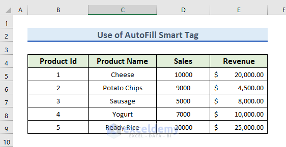
- Here, we have used the range B4:E9 to insert the sales information.
- Secondly, using the File tab, open the Excel Options window.
- After that, uncheck Show Paste Options button when content is pasted.
- Click OK to proceed.

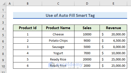
- Suppose, now we want to write the information about Ready Rice once again.
- So, select Cell C10 and type R.
- In the meanwhile, it can be noticed that Ready Rice is already showing in the cell.
- You have to just press ENTER.

- We will now fill up the other information according to our own choice and our output is ready.
4. Avail Insert Smart Tag to Insert Cells
Sometimes, it is necessary to insert some rows and columns in the dataset. By using the Insert smart tag, it can be possible to easily insert rows and columns with various kinds of smart modifications. Let’s follow the method to learn the procedure.
STEPS:
- First of all, you need to make the dataset ready.
- To do so, insert the data in an Excel sheet.
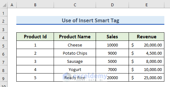
- Here, we have used the range B4:E9 to insert the sales information.
- From the File tab, open the Excel Options window and check the option named Show Insert Options buttons.
- After checking, select OK.

- Now, select the rows or columns you want to insert more information.
- We have selected the Sales and Revenue columns.

- Right-click on the mouse.
- Select Insert from the dialog box.

- As we want to insert a column here, we will select Entire column and press OK.

- After that, 2 columns appeared as we selected 2.
- A smart tag can be seen at the bottom of the newly formed columns.
- From the smart tag, we can select the formatting we want to keep for our newly formed columns.
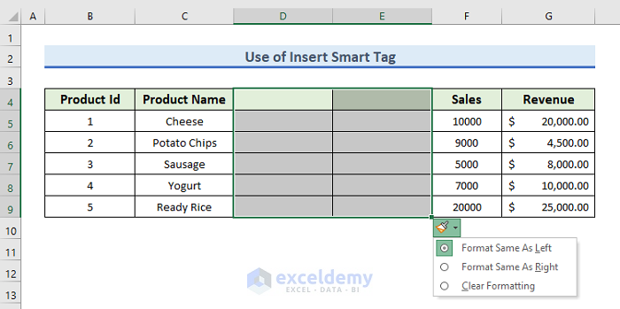
- We have selected Format Same As Left and the columns format remains unchanged.
- Finally, fill up the columns and make your updated dataset ready.

Read More: How to Use Multiple Tags in One Cell in Excel
5. Use Error Checking Smart Tag to Ignore Errors
Making errors is common to users. For this reason, it is helpful if we include Error Checking smart tags. We can include this tag and also remove it if it causes problems for the user. Let’s follow the method to learn the procedure.
STEPS:
- First of all, you need to make the dataset ready.
- To do so, insert the data in an Excel sheet.
- Here, we have used the range B4:E9 to insert the sales information.

- From the File tab, open Excel Options window and tick the button named Enable background error checking.
- After ticking, select OK.

- We want to know more information about the dataset.
- We have summed up the Sales and Revenue columns to get the total information of the business.
- In the next step, we also want to know the average sales and revenue.
- Dividing total sales and revenue by 5, we will get the average value.
- But accidentally in the case of finding the average sales, we have divided the total sales by 0.
- But a number can not be divided by 0.
- As error checking smart tag is applied in this case, the cell is showing a message that this cell contains an error.
- By seeing the message, we can be notified that we have made a mistake and should recheck the formula.

6. Apply Flash Fill Smart Tag to Fill Pattern in Excel
Flash Fill smart tag helps identify the formula you are trying to write and fills the cells accordingly. Let’s follow the method to learn the procedure.
STEPS:
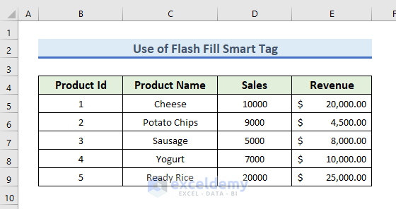
- First of all, you need to make the dataset ready.
- To do so, insert the data in an Excel sheet.
- Here, we have used the range B4:E9 to insert the sales information.
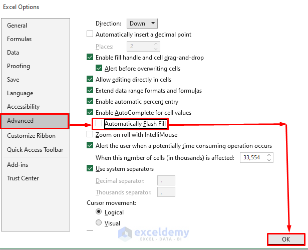
- From the File tab, open Excel Options window and tick the button named Automatically Flash Fill.
- After that, select OK.

- Suppose, we want to add a shortcode to each product.
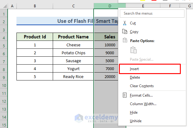
- For this reason, select the Sales column and right-click on the mouse.
- From the dialog menu select Insert.
- A new column will be shown up before the sales column and we will name the column Short Code.
- Type the first shortcode.
- We want that product’s shortcode to be its first two words.
- Type the 1st short code as Ch.
- Start typing the 2nd shortcode as P and you will notice that the other product’s name starts to show.
- Press Enter.
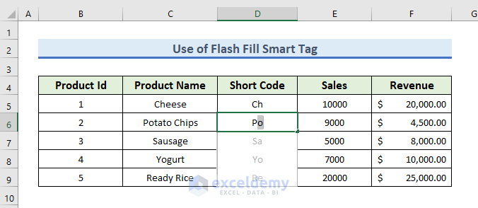
- After that, a flash fill smart tag starts to be shown.
- Click on Accept suggestions to fill up the excel automatically.

- To disable the Flash Fill smart tag, untick the Automatically Flash Fill and its operation will be turned off.
Read More: How to Create Price Tags in Excel
7. Utilize Quick Analysis Smart Tag for Different Excel Operations
According to the dataset, we can do some analysis with the help of Quick Analysis Smart Tag. Let’s follow the method to learn the procedure.
STEPS:
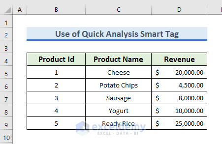
- Firstly, you need to make the dataset ready.
- To do so, insert the data in an Excel sheet.
- Here, we have used the range B4:D9 to insert the sales information.
- From the File tab, open Excel Options window and tick the button named Show Quick Analysis options on selection.
- After that, select OK.

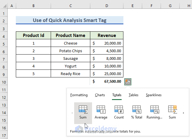
- To do the analysis of revenue, select the column of revenue.
- After selection, a quick analysis smart tag appears below the selection.
- Now, we have to select which type of analysis we want to do.

- If we want to sum the revenue, from the Totals tab press on the sum.
- At the bottom of the revenue column, the total revenue is shown.
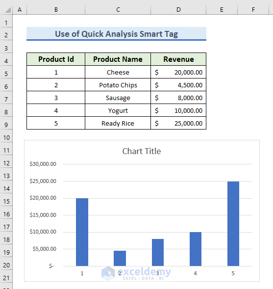
- If you want to make a chart of the revenue, select the chart type from Charts.
- Suppose, we want to see a clustered chart.
- So, select clustered and a floating chart can be seen.
- If this is our desired chart, press ENTER.

- Finally, this is our desired analysis and we have done that with the Quick Analysis smart tag.
Read More: How to Filter Tags in Excel
Download Practice Workbook
To practice by yourself, download the following workbook.
Conclusion
In this article, we have demonstrated the way to use smart tags in Excel. There is a practice workbook at the beginning of the article. So, go ahead and try the smart tags in Excel. Last but not least, please use the comment section below to post any questions or make any suggestions you might have.
Related Articles
<< Go Back to Tags in Excel | Data Analysis with Excel | Learn Excel
Get FREE Advanced Excel Exercises with Solutions!
