In this article, we will demonstrate how to create price tags in Excel with sample data columns. You can adapt the data according to your needs.
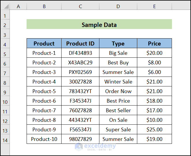
Suppose we have a sample dataset containing columns for Product, Product ID, Type, and Price. We will have to add extra columns to create price tags for the products from this data.
Step 1 – Add Extra Columns to Join the Text
For our price tags, we will create columns with Title and Value side by side like the following:
Product: Product-1
Product ID: DF434893
Type: Big Sale
Price: $20
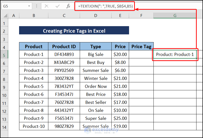
To do so, we’ll use the TEXTJOIN function to combine Row 4 with the corresponding data in the other rows.
- Enter the following equation in cell G5:
=TEXTJOIN(": ",TRUE,$B$4,B5)Here,
“: ” = The delimiter Argument
TRUE = Ignore Empty Cells
$B$4 = Product
B5 = Product-1
Result: Product: Product-1
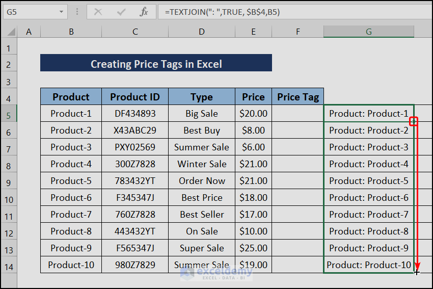
- Press Enter.
- Drag the Fill Handle downwards to complete the series.
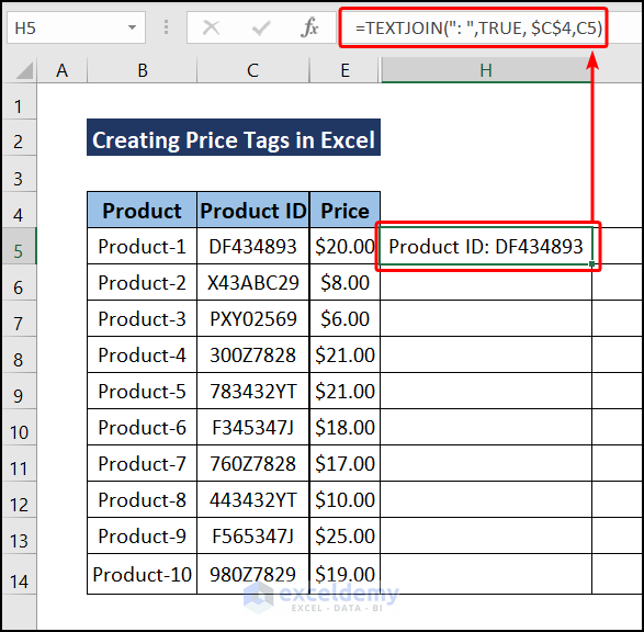
Now we can use the TEXTJOIN function to combine Row 4 with the corresponding data in the other rows.
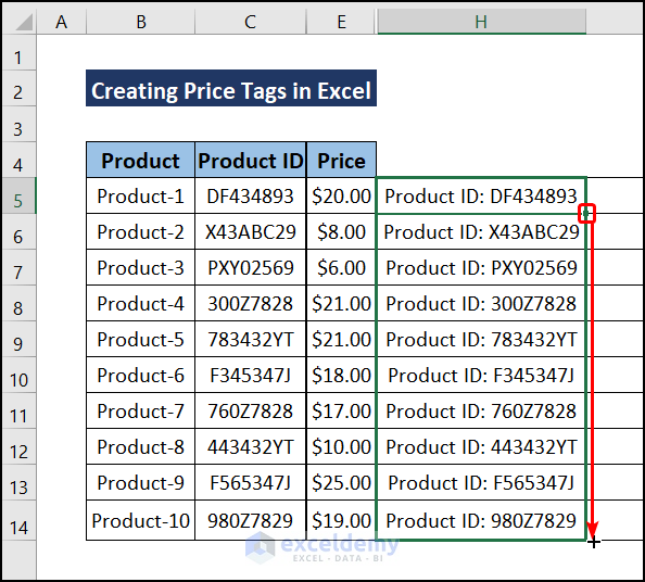
- Enter the following formula in cell H5:
=TEXTJOIN(": ",TRUE,$C$4,C5)Here,
“: ” = The delimiter Argument
TRUE = Ignore Empty Cells
$C$4 = Product ID
C5 = DF434893
Result: Product ID: DF434893
- Press Enter.
- Drag the Fill Handle downwards to complete the series.
Then we again use the TEXTJOIN function to combine Row 4 with the corresponding data in the other rows.
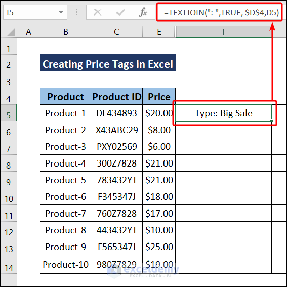
- Enter the following equation in cell I5:
=TEXTJOIN(": ",TRUE, $D$4,D5)Here,
“: ” = Delimiter Argument
TRUE = Ignore Empty Cells
$D$4 = Type
D5 = Big Sale
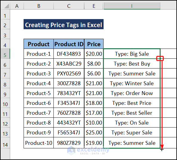
Result: Type: Big Sale
- Press Enter.
- Drag the Fill Handle downwards to complete the series.
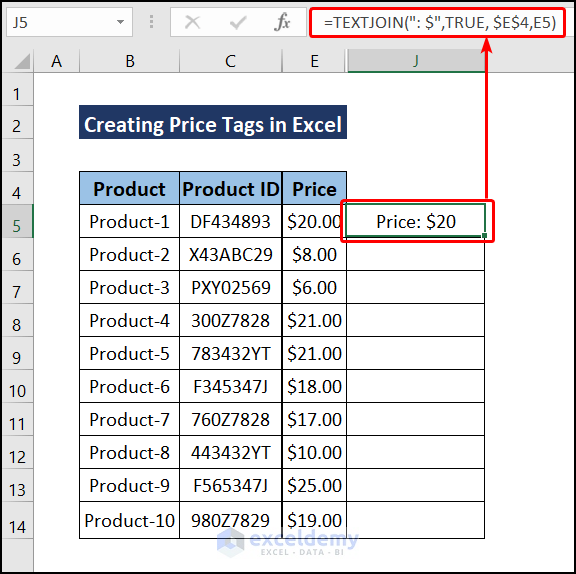
In the last column, we will use the TEXTJOIN function to combine Row 4 with the corresponding data in the other rows.
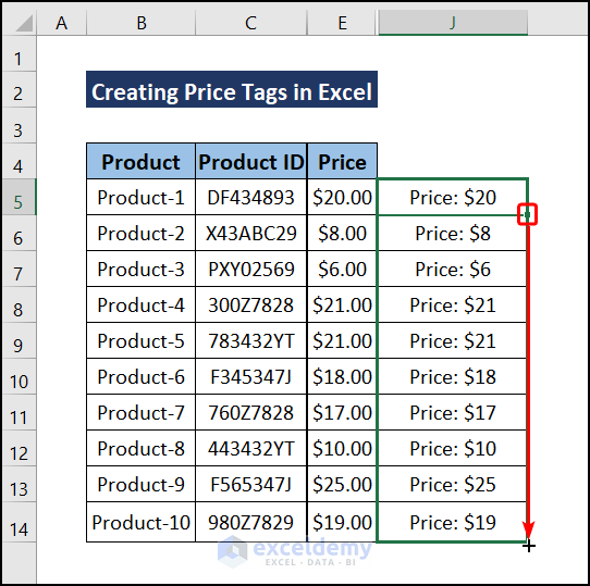
- Enter the following equation in cell J5:
=TEXTJOIN(": $",TRUE, $E$4,E5)Here,
“: $” = Delimiter Argument
TRUE = Ignore Empty Cells
$E$4 = Price
E5 = $20
Result: Price: $20
- Press Enter.
- Drag the Fill Handle downwards to complete the series.
Step 2 – Create Price Tags Within a Cell
Now we can combine the cells from the extra columns into the Price Tag.
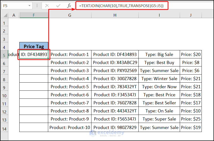
- In cell F5, enter the following formula:
=TEXTJOIN(CHAR(10),TRUE,TRANSPOSE(G5:J5))Here,
CHAR(10) = Line Break Argument
TRUE = Ignore Empty Cells
TRANSPOSE(G5:J5) = Cells from G5 to J5 will be transposed.
Result: “Product: Product-1
Product ID: DF434893
Type: Big Sale
Price: $20″
- Press Enter.
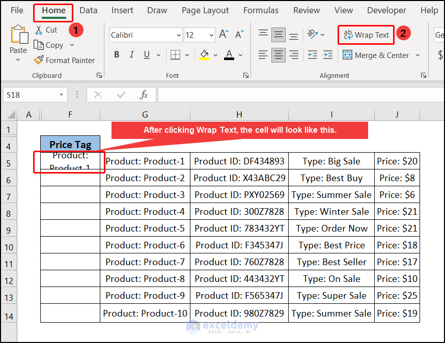
- Select cell F5.
- Go to Home >> Alignment >> Wrap Text.
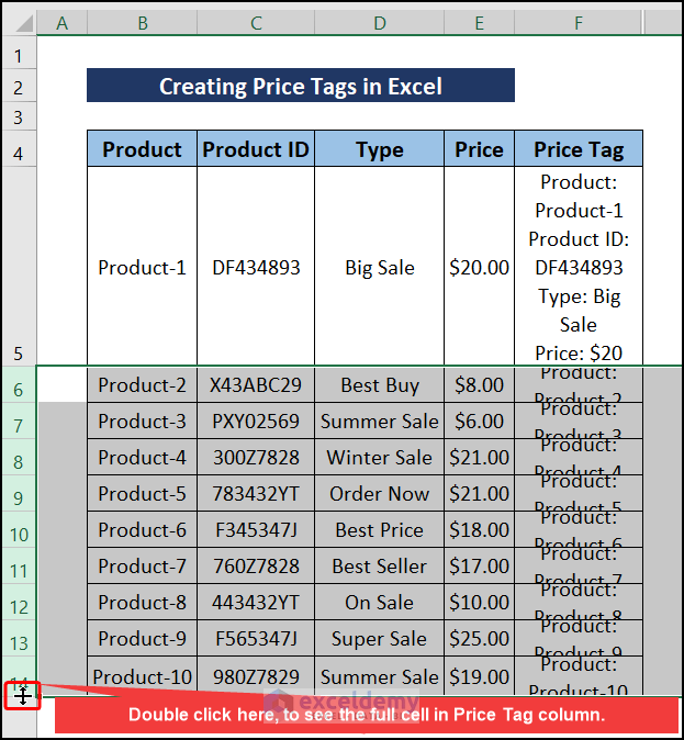
- To see the full cell, double-click on the row like in the image below (or use the AutoFit Row Height command).
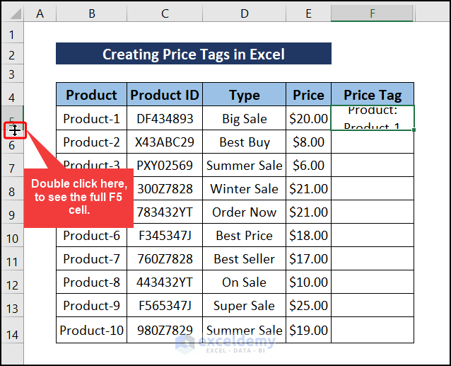
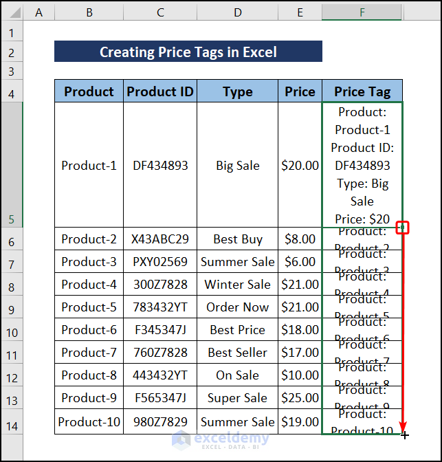
- To complete the Price Tag column, drag the Fill Handle down like in the image below.
- Select multiple rows.
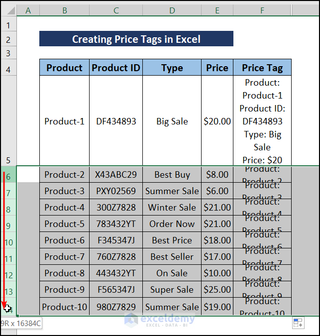
- Double-click on the mouse when the Excel cursor changes shape as in the following image.
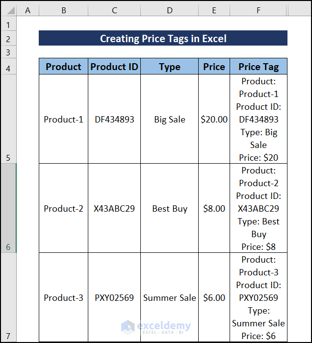
All the row heights adjust to Autofit the contents.
- Modify the tag as desired.
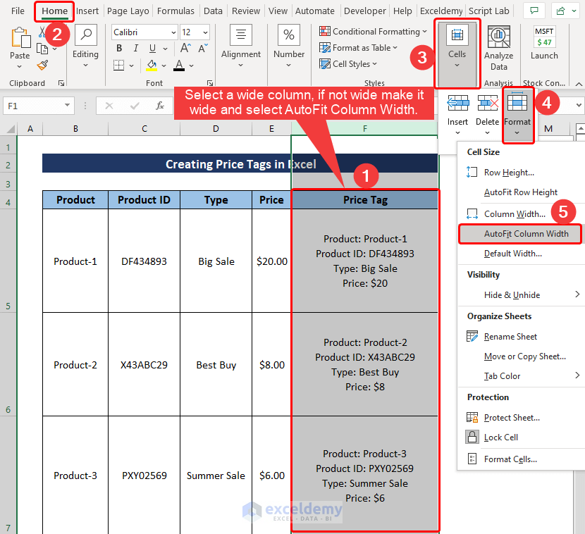
- Select a wide column. If its not wide, widen it.
- Select AutoFit Column Width.
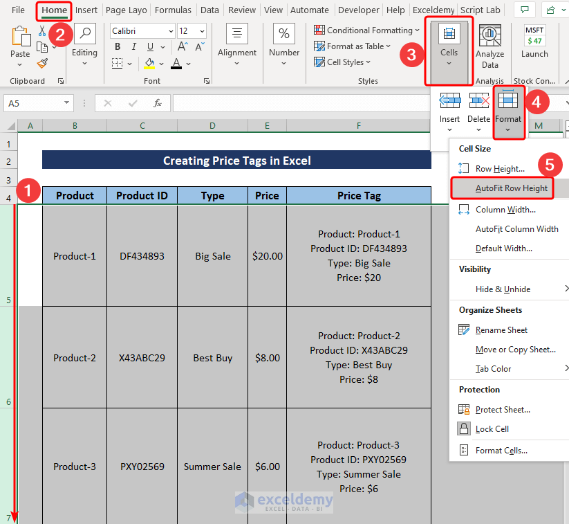
- Select all rows and select AutoFit Row Height.
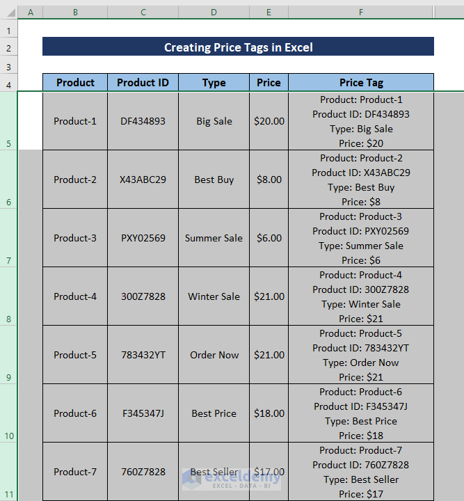
Our final table containing data for the price tags is as in the image below.
Download Practice Workbook
Related Articles
- Smart Tags in Excel: Definition & Different Uses
- How to Add Tags in Excel
- How to Add Tag to Properties in Excel
- How to Use Multiple Tags in One Cell in Excel
- How to Filter Tags in Excel
<< Go Back to Tags in Excel | Data Analysis with Excel | Learn Excel
Get FREE Advanced Excel Exercises with Solutions!
