How to Reduce Decimals in Excel (10 Easy Methods)

To reduce decimal points in Excel:

Select the cell where you want to decrease decimal points.
Go to Home tab > Number group > Decrease Decimal.

Now, you will see that decimal points have been decreased.

Method 1 – Using the Decrease Decimal Button

Steps:

Select a range of cells.
Go to Home tab > Number group > Decrease Decimal button.
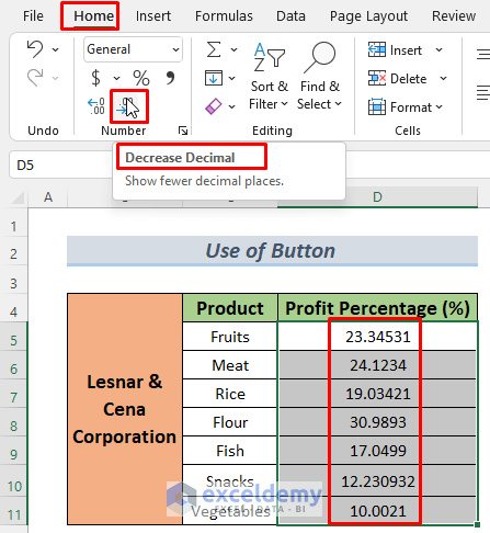
Click on the button one or multiple times. This will reduce the decimals in your selected data range.

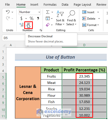
Note: Reducing the number of decimal places using the Decrease Decimal button does not change the underlying values in the cells; it only changes how the numbers are displayed. The actual precision of the numbers remains unchanged.

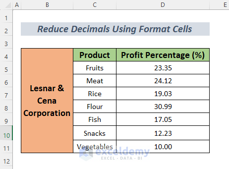
Method 2 – Using a Format Cells Dialog Box

Steps:

Select a range of cells.
Press Ctrl+1 to open the Format Cells dialog box.
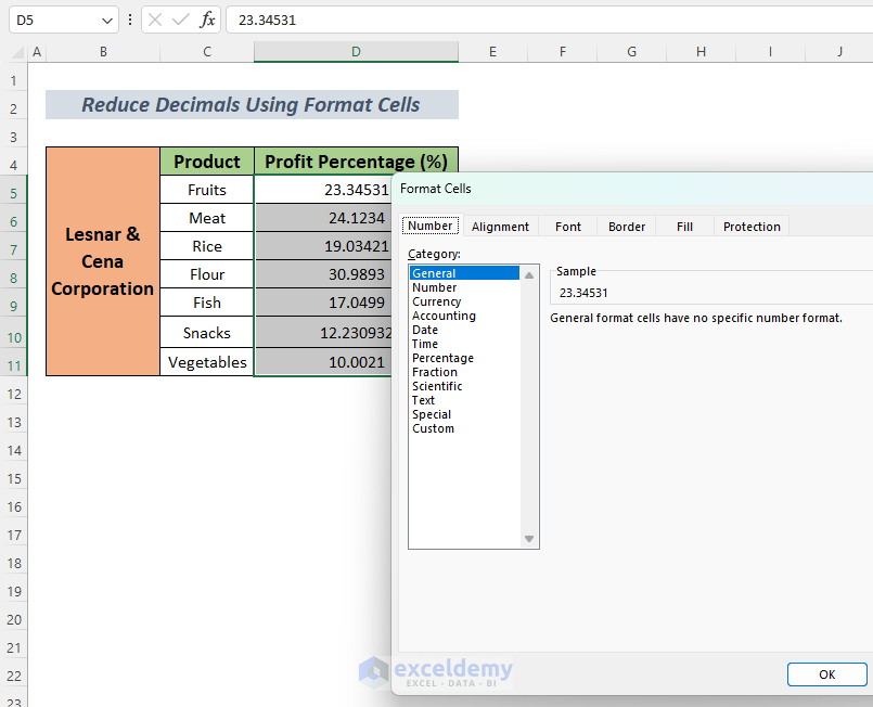
In the Format Cells dialog box:
- Choose Accounting/Currency/Percentage/Scientific from Category based on your data type.
- Put the desired number in the Decimal places box.
  Here, I have entered 2.
- Click OK.

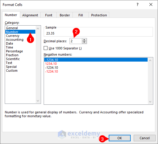
This will reduce the decimals to 2 places in your selected cells.

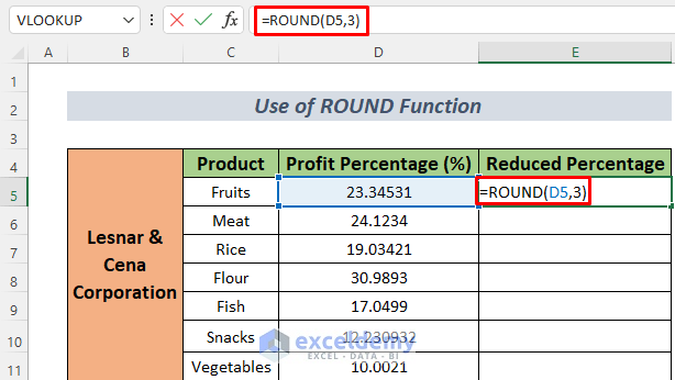
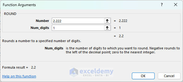
Method 3 – Applying the ROUND Function

Steps:

Select the cell where you want to decrease decimal points.
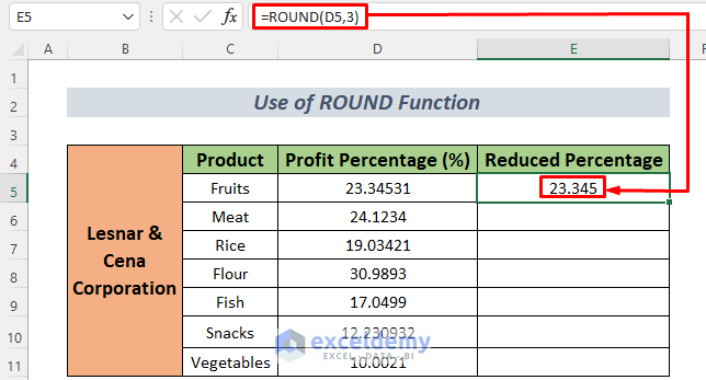
Insert the following formula: =ROUND(D5,3)
Here, D5 represents the cell with decimal value and 3 indicates the number of desired decimal places. Replace these arguments with your required values.
Press the Enter key to see the reduced decimal value.
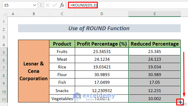
Use the Fill Handle to copy the formula in the remaining cells.

Note: You can also find the ROUND function from Formulas > Math & Trig > ROUND. When the Function Argument window opens, enter the cell reference or number for which you want to reduce the decimal and the number of decimal places you want in the Number and Num_digits boxes, and press OK.

Method 4 – Using the ROUNDUP Function

Steps:

Select the cell where you want to decrease decimal points.
Inset the formula: =ROUNDUP(D5,2)
Here, D5 represents decimal value and 2 represents desired decimal places. Replace these arguments with your required values.
Press Enter.
This will reduce the decimal places.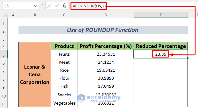
Drag the Fill Handle icon to copy the formula in the remaining cells.

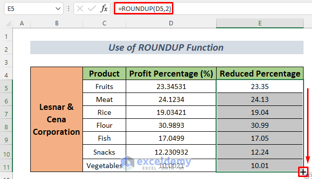
Thus, you can reduce decimals from a number in Excel using the ROUNDUP function.

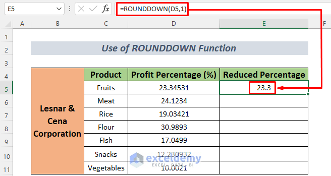
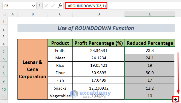
Method 5 – Applying the ROUNDDOWN Function

Steps:

Select the cell where you want to decrease decimal points.
Inset the formula: =ROUNDDOWN(D5,1)
Here, D5 represents the cell with decimal value and 1 indicates the number of desired decimal places. Change these arguments with your required values.
Press Enter.
Now you will see the reduced decimal value in the selected cell.
You can copy the formula in the remaining cells using the Fill Handle tool.

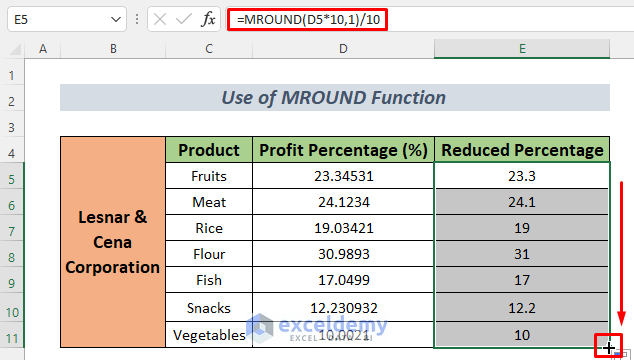
Method 6 – Using the MROUND Function

Steps:

Select the cell where you want to decrease decimal points.
Inset the formula: =MROUND(D5*10,1)/10
Here, D5 is the decimal data, and 1 sets the rounding interval, like rounding to the nearest whole number when divided by 10. You can replace these values with your desired multiple.
Press the Enter key to see the reduced decimal value.
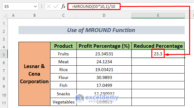
Drag the Fill Handle icon to copy the formula in the remaining cells.

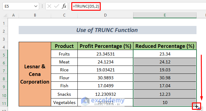
Method 7 – Using the TRUNC Function

Steps:

Select a cell.
Inset the formula: =TRUNC(D5,2)
Here, D5 is the cell with decimal points and 2 is the decimal points that will remain.
Press Enter.
This will reduce the decimal value.
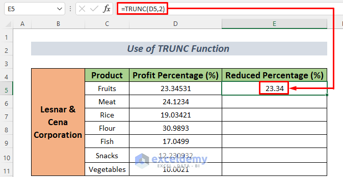
Drag the Fill Handle icon to fill the remaining cells.

Method 8 – Applying the INT function

Steps:

Select the cell where you want to decrease decimal points.
Inset the formula: =INT(D5*1000)/1000
Here, D5 is the decimal data, and 1000 represents the multiplier for rounding to 3 decimal places (as 10³ = 1000).
Press Enter.
You will see the reduced decimal value in the selected cell.
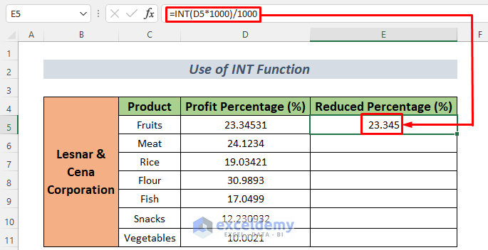
Drag the Fill Handle icon down to fill the remaining cells.

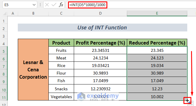
Note: The INT function makes a negative number more negative by rounding it down. For example, if you use =INT(-33.456), the INT function will return -34.

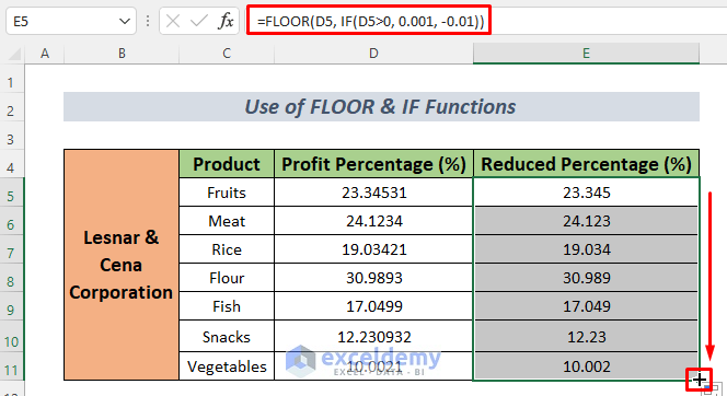
Method 9 – Combining IF and FLOOR Functions

Steps:

Select the cell where you want to decrease decimal points.
Inset the formula: =FLOOR(D5, IF(D5>0, 0.001, -0.01))
Here, D5 is the decimal value, and the formula rounds it down to the nearest smaller multiple of 0.001 if positive or to the nearest smaller multiple of -0.01 if negative. Change the cell reference and multipliers according to your required values.
Press Enter to get the reduced decimal value.
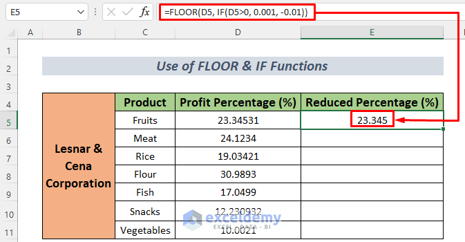
Drag the Fill Handle icon to copy the formula in the remaining cells.

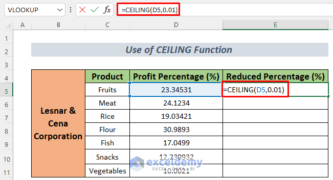
Method 10 – Using the CEILING Function

Steps:

Select the cell where you want to decrease decimal points.
Inset the formula: =CEILING(D5,0.01)
Here, D5 is the decimal number you want to round up, and 0.01 is how much you want to round it up by.
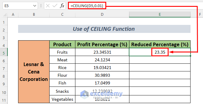
Press the Enter key.
You will see the reduced decimal value.
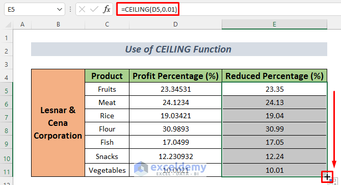
You can copy the formula in the remaining cells using the Fill Handle.

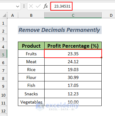
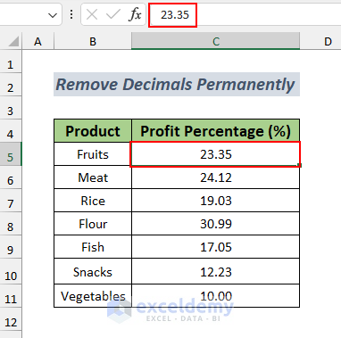
How to Remove Decimals Permanently

If you reduce decimals using the Decrease Decimals or Format Cells feature in Excel, only the displayed value will change, and the actual precision of the numbers will remain unchanged.

Steps:

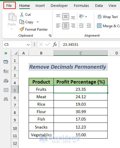
Go to File.
Select Options.
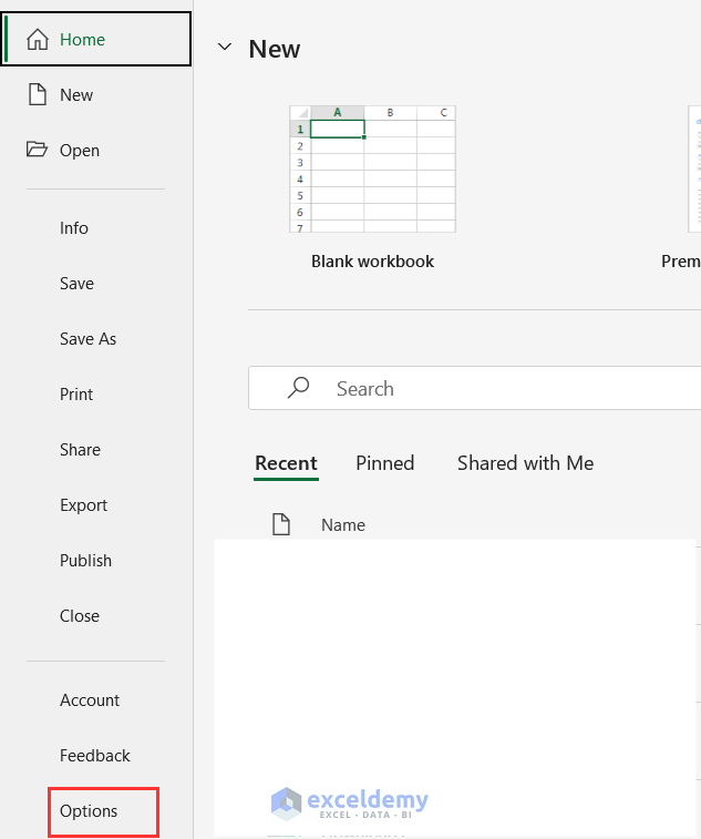The Excel Options window will open.
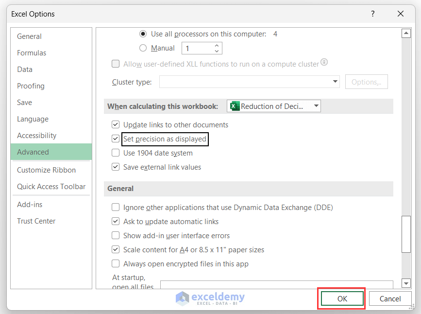
In the Excel Options window:
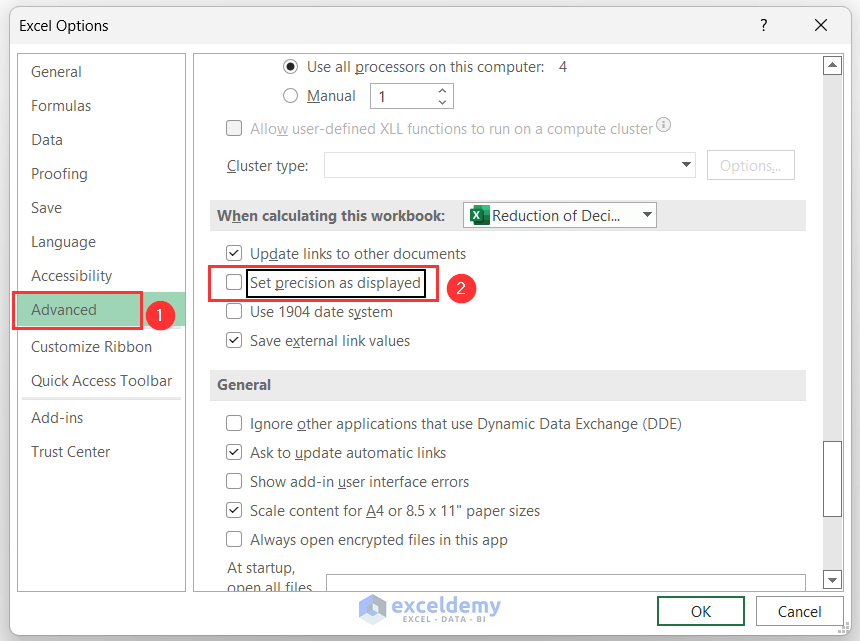
- Select the Advanced from the left-side pane.
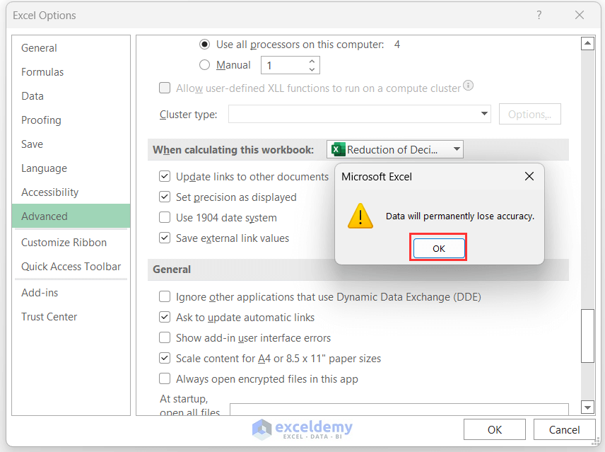
- Enable the Set precision option as displayed when calculating this workbook.A message box will appear to ensure your last change.
- Press OK.
In the Excel Options window, click OK.
This will take you to the worksheet.
Select the range with decimals and click the Decrease Decimals button or use the Format Cells dialog box to reduce decimals, you will notice that the cell value and formula bar value are equal.