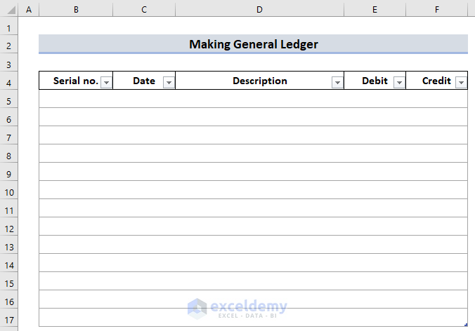
Step 1 – Input Fields and Choose the Range
- Select data to input into the General Ledger. A typical ledger has 5 fields: Serial no., Date, Description, Debit, and Credit.
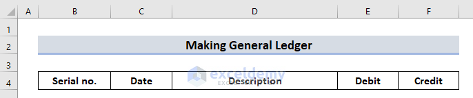
- Bold the names and increase the font size in the headers.
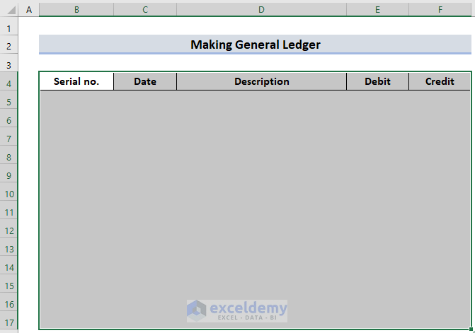
Step 2 – Creating a Pivot Table
Here, 13 rows will be inserted.
- Select B4:F17.
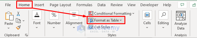
- Go to the Home tab and select Format as Table. Choose a type of table.
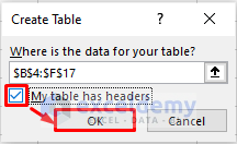
- In the confirmation box, check My table has headers.
- Click OK.
The table will be displayed.
- Select Borders and go to Line Style.
- A thick line border was selected here.
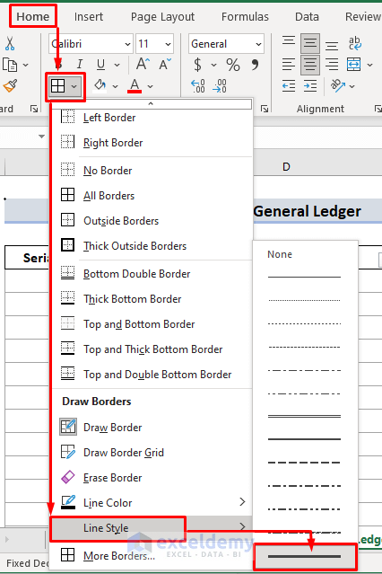
- Draw lines and separators.
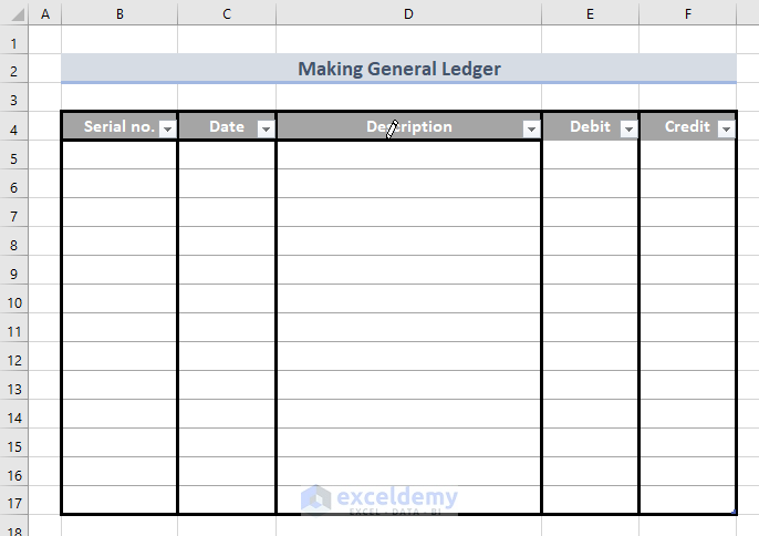
- Select the entire table and go to Table Design.
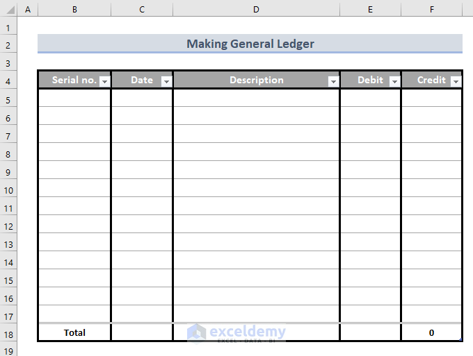
- Select Total Row to display a Total row at the end of the table.
- Use Line Border for this row.
Step 3: Entering Calculation Functions in Table
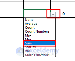
- Click the last cell in Debit. Here, E18.
- Click the small arrow on the right.
- Select Sum.
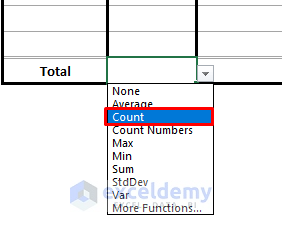
- In total days, select C18 and choose Count.
This is the output.
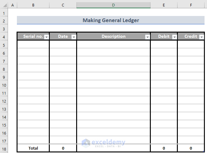
Since there is no data in the table, the total field is showing 0.
Step 4: Analyzing the General Ledger
- Enter data.
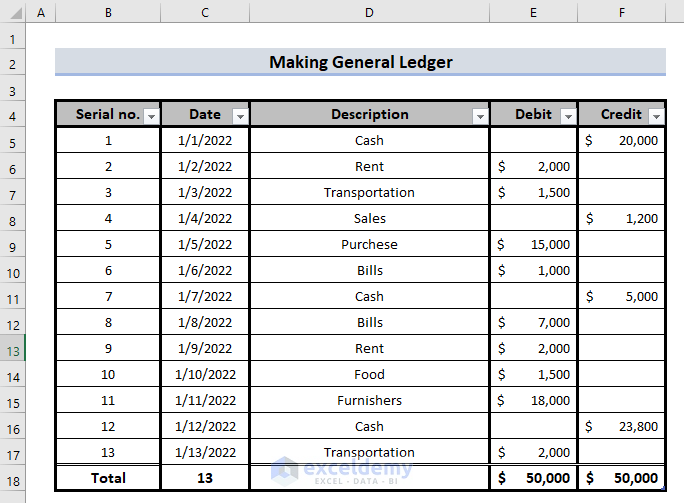
The Debit and Credit data type is selected as Accounting.
To see the amounts of Debit or Credit for each description:
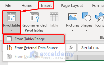
- Select the entire table and go to Insert.
- Select From Table/Range in Pivot Table.
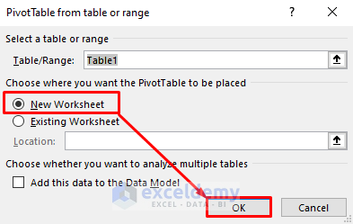
- In the dialog box, select New worksheet and click OK.
A new sheet containing the Pivot Table field panel on the right will be displayed.
- Select the fields.
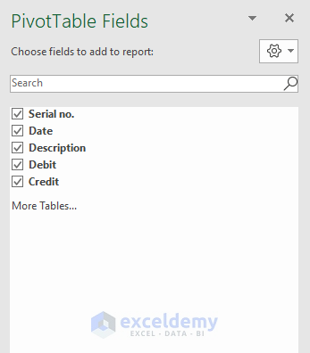
- Here, Description to categorize based on Description, Debit, Credit, and other fields.
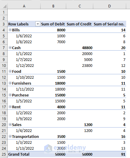
This is the output.
Read More: How to Make a Bank Ledger in Excel
Download Practice Workbook
Download the practice workbook here.
Related Articles
- How to Make Subsidiary Ledger in Excel
- Export All Ledgers from Tally in Excel
- How to Make a Ledger in Excel
- How to Maintain Ledger Book in Excel
- How to Create a Checkbook Ledger in Excel
- Create General Ledger in Excel from General Journal Data
<< Go Back to Ledger in Excel | Excel for Accounting | Learn Excel
Get FREE Advanced Excel Exercises with Solutions!
