How to Maintain Ledger Book in Excel (with Easy Steps)

An Overview of a Ledger Book

An accounting ledger book records all transactions and financial statements of a company. Under the general ledger account, the balance sheet is organized into multiple accounts such as assets, accounts payable, accounts receivable, stockholders, equities, liabilities, taxes, revenues, expenses, funds, loans, profit, loss, stocks, bonds, wages, etc.

Ledger books usually come in three types:

Sales Ledger

A sales ledger is a record of the sale of goods or services to customers. It allows companies to create income statements.

Purchase Ledger

The Purchase Ledger records a company’s transactions when purchasing goods, services, or products from other organizations. It’s vital in keeping track of expenses.

General Ledger

Nominal Ledger: The nominal ledger provides us with information on earnings, expenses, insurance, depreciation, etc.
Private Ledger: The private ledger keeps track of confidential information such as salaries, wages, capital, etc.

Read More: How to Make a Ledger in Excel

How to Maintain a Ledger Book in Excel: Step-by-Step Procedure

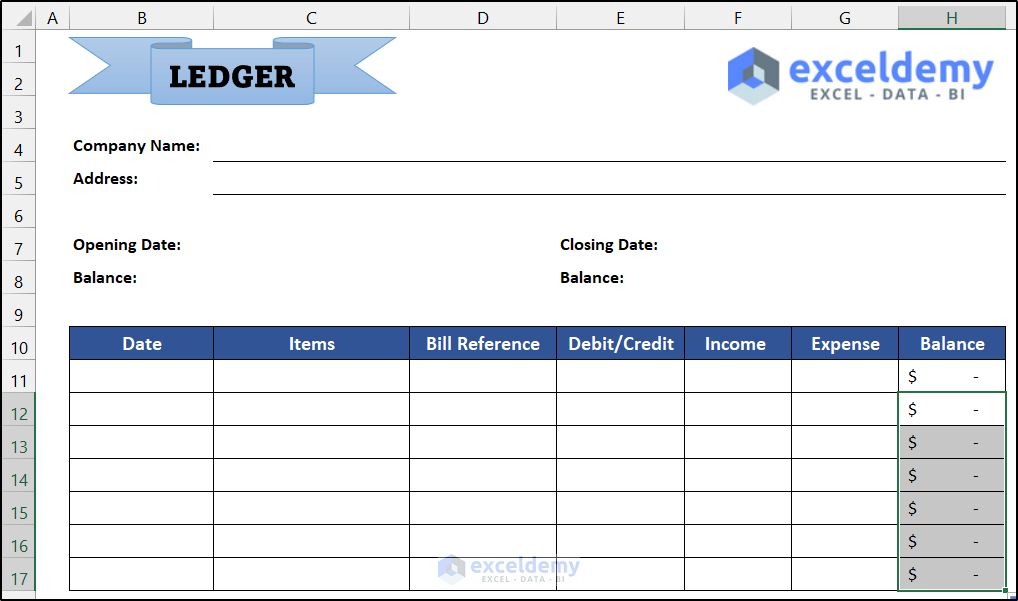
Step 1 – Create a Layout of the Ledger Book

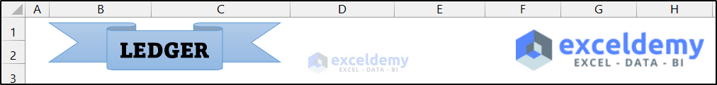
In the Insert tab, click on Illustration and select the Shapes option.
Select a shape for the header. We chose Ribbon: Tilted Down shape.

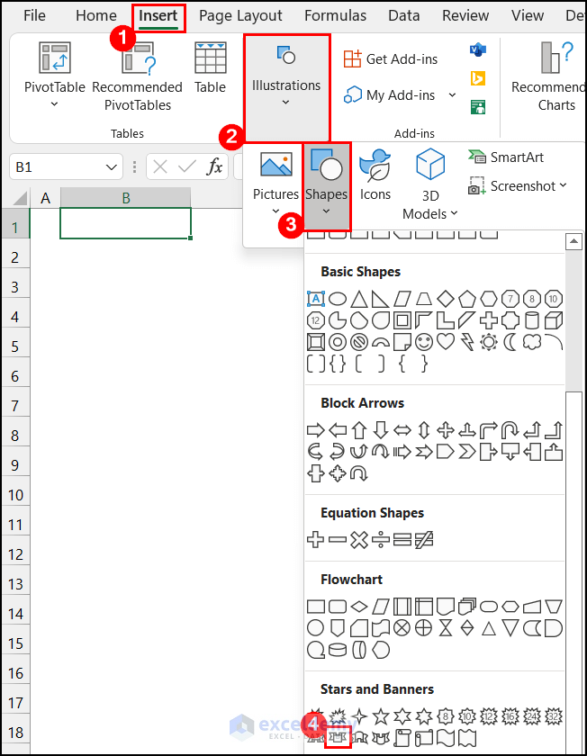
Your mouse cursor icon will change. Click and drag your mouse over the sheet to draw the shape.
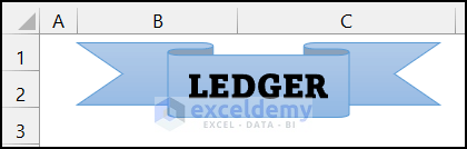
Insert the title as LEDGER.

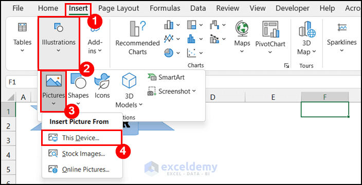
Select cell F1, and in the Insert tab, click on Illustration and select the Pictures option.
Choose the This Device option.

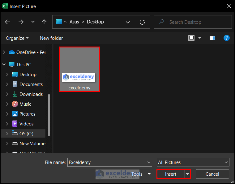
A small dialog box called Insert Picture will appear.
Select your organization’s logo and click the Insert button. We chose our website’s logo to demonstrate the process.

Place the logo at a suitable location on the sheet.

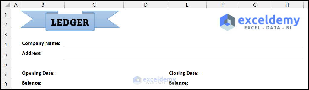
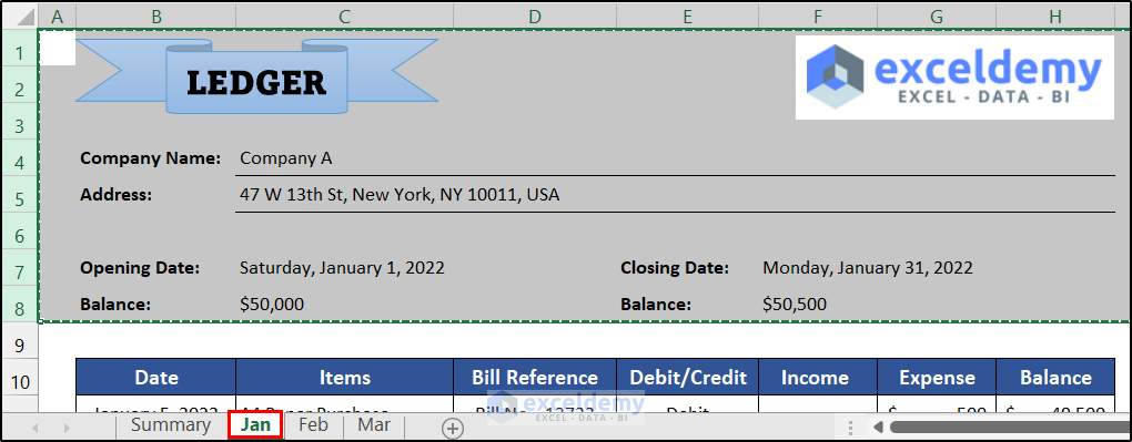
In the range of cells B4:B5, B7:B8, and E7:E8, write down the basic company and ledger information and format the corresponding cells as the input cells of these values.

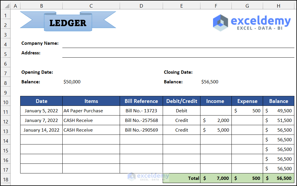
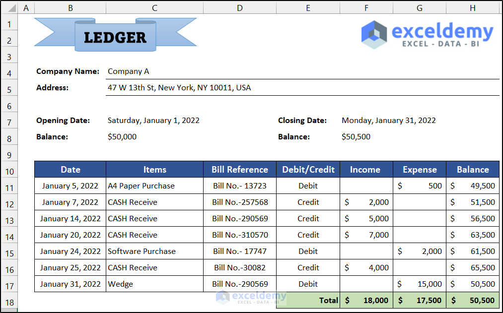
Step 2 – Generate a Ledger Book for Each Month

In the range of cells B10:H10, insert the following column headers.

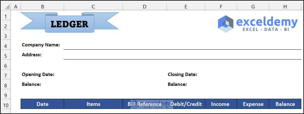
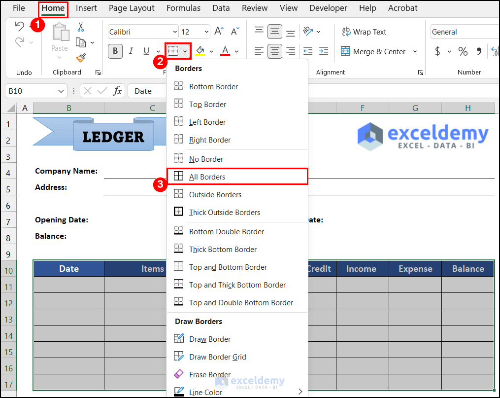
Let’s assume that we have 7 financial activities each month. We selected the range of cells B10:H17 as our ledger book dataset and formatted the cells with the All Border option from the Font group located in the Home tab.

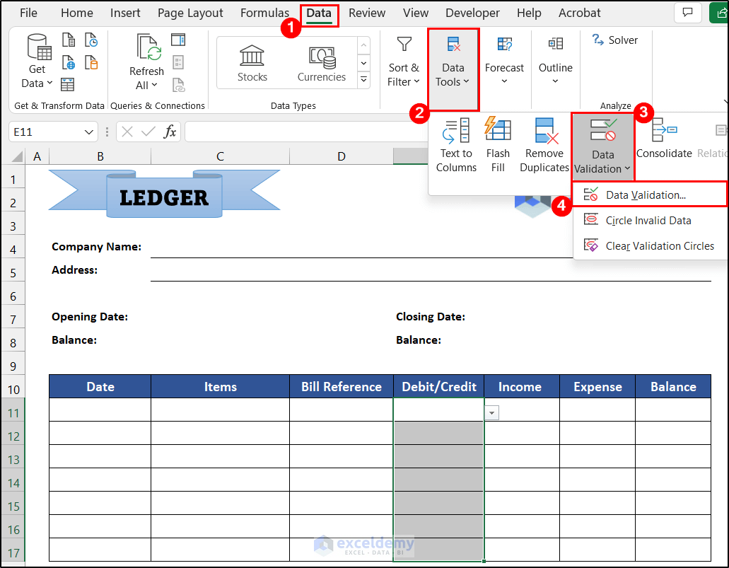
We need a data validation option in column H. When a person uses this ledger, they can only input either Debit or Credit in the range of cells H11:H17.
Select the range of cells H11:H17, and in the Data tab, click Data Validation and select Data Validation from the group Data Tools.

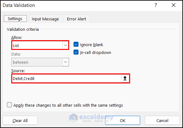
The Data Validation dialog box will appear.
Change the Allow field from Any value to List, and in the Source field, write down “Debit,Credit“.
Click OK.

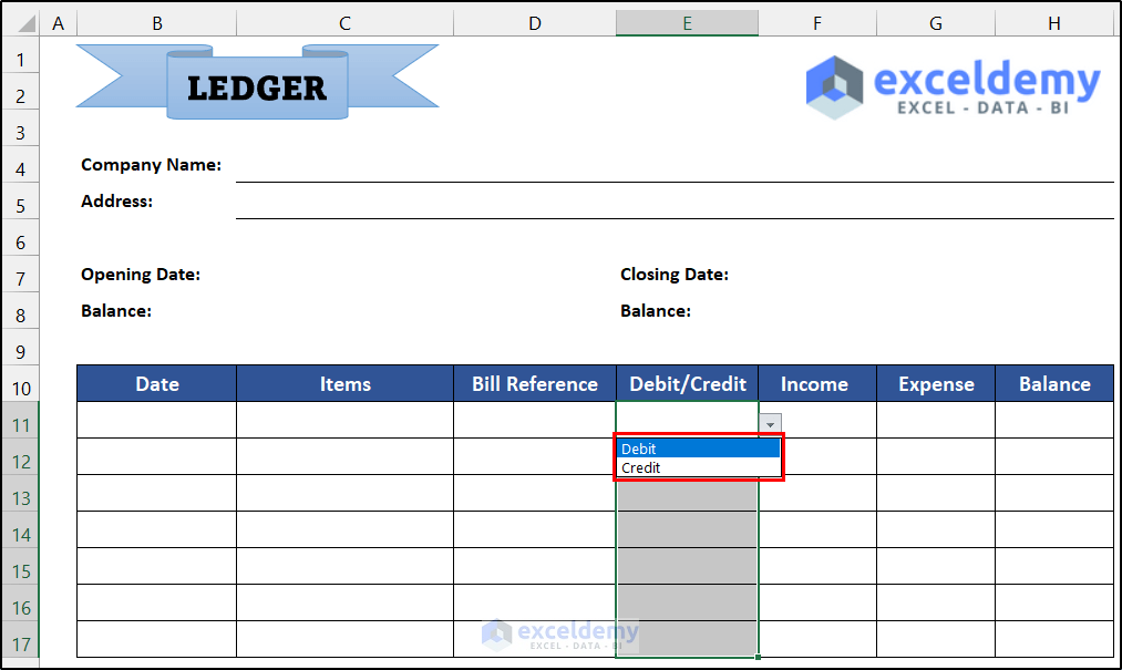
You will find the data validation drop-down at those cells.

Insert the following formula into cell H11.

=C8+F11-G11

Press Enter.

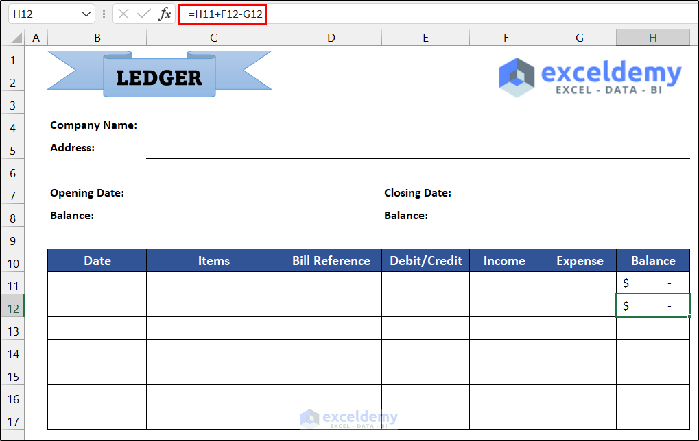
Insert the following formula into H12.

=H11+F12-G12

Press Enter.

Drag on the Fill Handle icon to copy the formula from H12 down to cell H17.

Use the following formula in cell F18.

=SUM(F11:F17)

Press Enter.

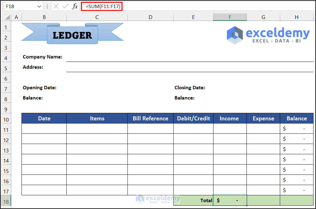
Drag the Fill Handle from F18 to G18.
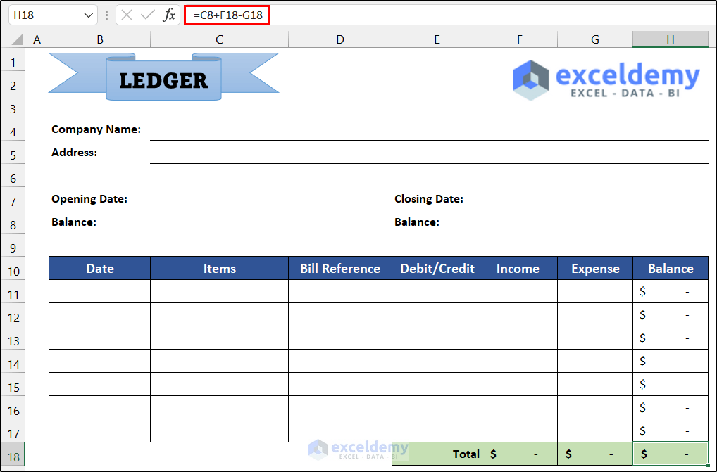
Use the following formula in cell H18.

=C8+F18-G18

Press Enter.

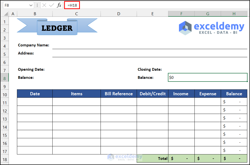
Input the following formula in the merged cell F8.

=H18

Press Enter.

Insert sample data to ensure all of the formulas are working accurately in this sheet.

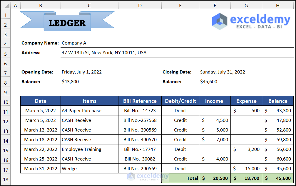
Create more sheets for the subsequent months, February and March.

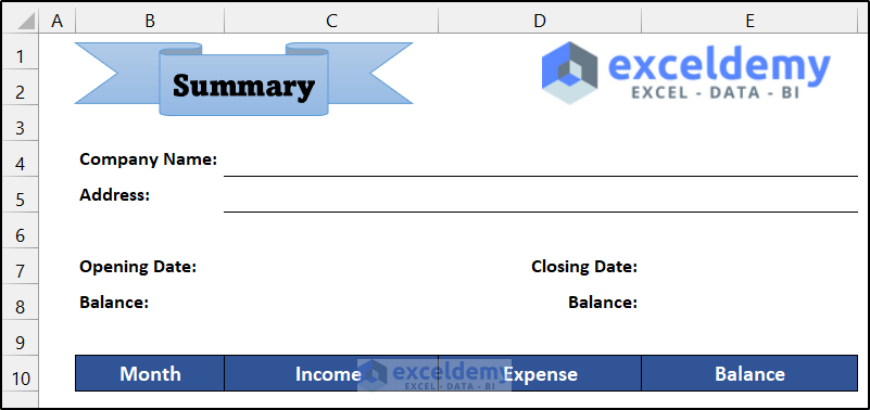
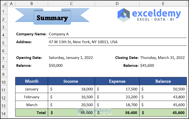
Step 3 – Design Summary Report

Select rows 1:8 in the Jan sheet and press Ctrl + C to copy.

Go to the Summary sheet and press Ctrl + V to paste.

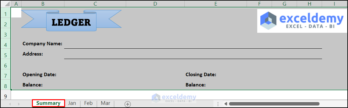
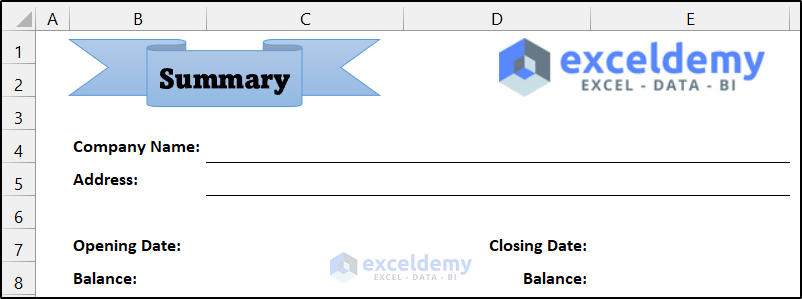
Change the sheet title from LEDGER to Summary.
We will show the month’s name, income, expense, and balance in the Summary sheet. Modify the information in four columns and delete all the unnecessary columns.

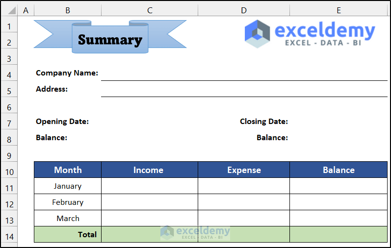
Insert the column headers in the range of cells B10:E10.

Insert month names in the range of cells B11:B13 and insert all borders to all the cells.
Denote row 14 as Total to show the total of all columns.

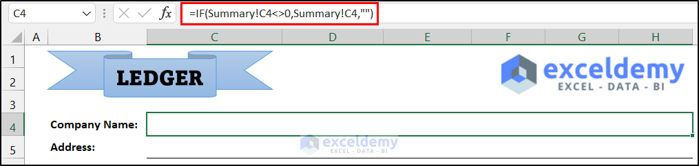
Step 4 – Establish a Relation Between Sheets

To get the company name from the Summary sheet to the Jan sheet, use the following formula in cell C4.

=IF(Summary!C4<>0,Summary!C4,"")

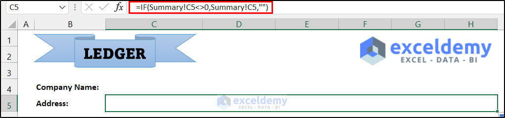
Press Enter.

Then, drag the Fill Handle icon in cell C5 to import the address from the Summary sheet.

Manually input the value for Opening Date, Opening Balance, and Closing Date in all sheets.
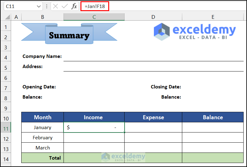
To get the total Income for January, use the following formula in cell C11.

=Jan!F18

Press Enter.

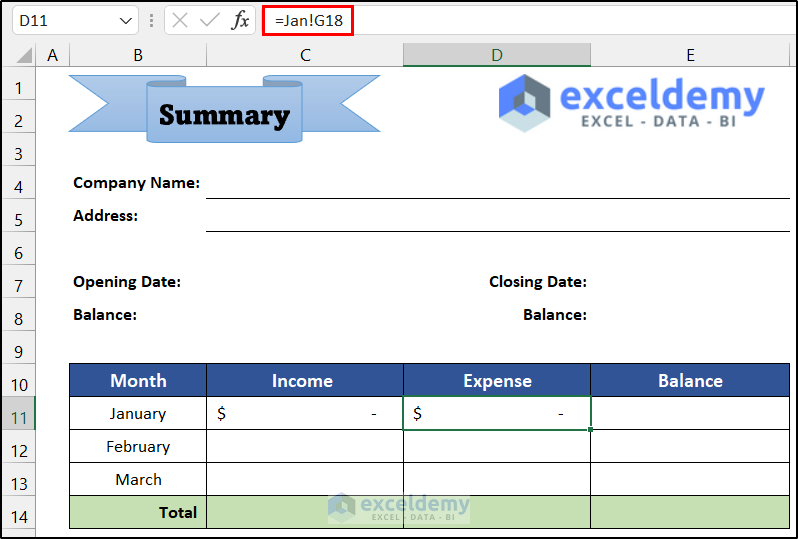
To import the total Expense for January, use the following formula in cell D11.

=Jan!G18

Press Enter.

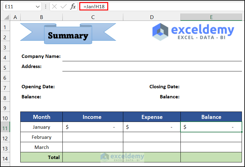
To get the final Balance for January, use the following formula in cell E11.

=Jan!H18

Press Enter.

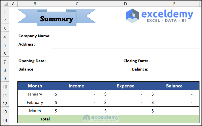
You will get all the values for January. Use similar formulas to import the total values for February and March.

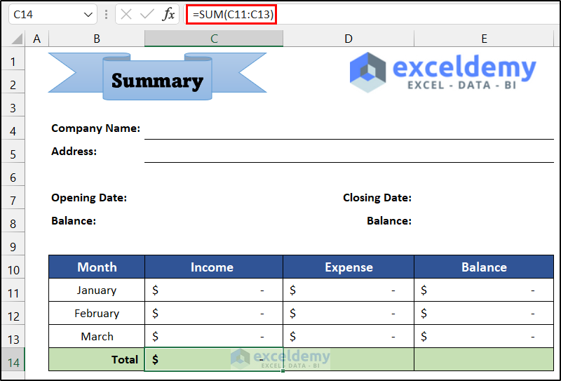
To get the quarterly Total Income, use the following formula:

=SUM(C11:C13)

Press Enter.

Use the SUM function to evaluate the total of the Expense column.
To get the total closing balance, use the following formula in cell E14.

=C8+C14-D14

Press Enter.

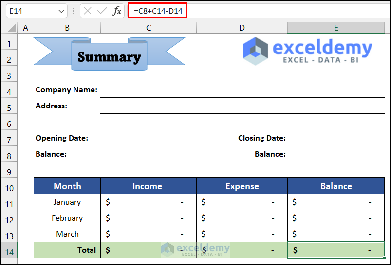
As this is a quarterly ledger book, the value of the Closing Balance will be the Closing Balance of March.
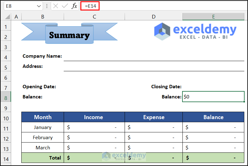
To show the value in cell E8, use the following formula for that cell.

=E14

Press Enter.

Step 5 – Verify the Ledger Book with Sample Data

Input the name of the company and address in the Summary sheet.

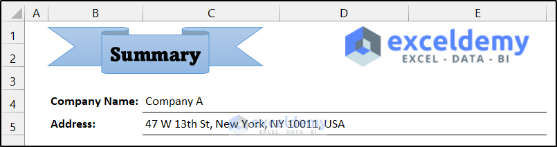
You will see that data exported in the other three sheets.
Input all the required data in the sheet titled Jan.

Input the sample data in the sheet entitled Feb.

Input the data in the sheet for March.

Go to the Summary sheet, and you should see imported data.

Download the Practice Workbook

Download this practice workbook that you can also use as a template. Insert the rows for more transaction records for each months and more sheets for further tracking. Make sure to modify the formulas as necessary.

Maintain Ledger Book.xlsx

<< Go Back to Ledger in Excel | Excel for Accounting | Learn Excel

Get FREE Advanced Excel Exercises with Solutions!