Basically, you may need to lock multiple cells for two reasons. One is to lock cells for protecting them from further edits or changes whereas the other reason is to use the locked cells as absolute cell references. In this instructive session, we’ll show you 6 methods on how to lock multiple cells that are applicable not only for protection but also for absolute reference in Excel.
How to Lock Multiple Cells in Excel: 6 Suitable Methods
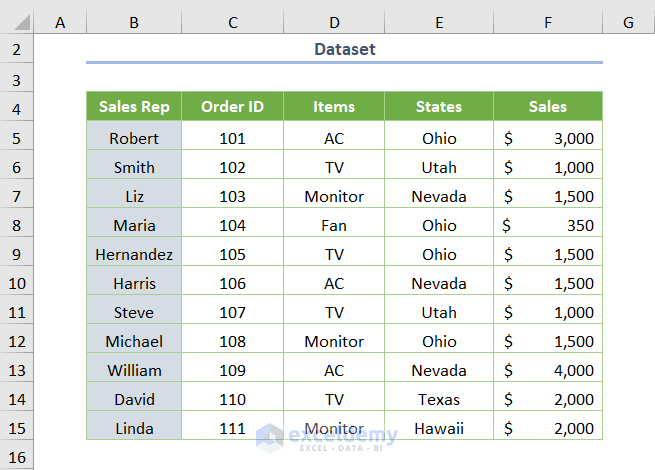
Today we’ll use the following dataset where the amount of Sales is provided along with their corresponding Sales Rep, Order ID, and so on. Now, we’ll see the application of the methods to lock multiple cells in Excel.
As we said earlier, you might lock the cells mainly to protect cells and use them as absolute references. So, you’ll see 4 methods to lock multiple cells to protect them first. Later, two effective methods including a shortcut method will be discussed to lock multiple cells.
Let’s dive into the methods.
How to Lock Multiple Cells to Protect Them: 4 Methods
Prior to applying the methods to lock multiple cells for protecting them, let us share an important thing. Actually, only locking cells don’t have any effect in Excel until you turn on the protection of the sheet. So, you must protect the sheet to get the output of locked cells.
1. Using the Format Cells Option
When you want to lock multiple cells in Excel to protect them, simply, you may lock any specific cells using the Format Cells option. Just follow the step-by-step process.
Step 01: Removing the Default “Locked” Option
Here, you should know that all cells are “locked” cells in Excel by default. Hence, when you want to lock specific multiple cells, you have to remove the default option.
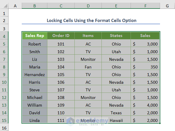
For this reason, select all cells within the dataset by pressing Ctrl + A only. Before doing that make sure that your cursor is in a cell within the dataset.
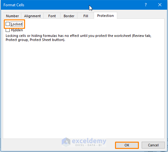
Now, open the Format Cells by pressing Ctrl + 1 easily or right-click and choose the option from the Context Menu.
Then, you’ll see that the box is checked before the Locked option (by default setting).
Therefore, you have to uncheck the box and press OK.
Step 02: Locking Specific Multiple Cells
Next, select the multiple cells (e.g. B5:F9 cell range) that you want to lock.
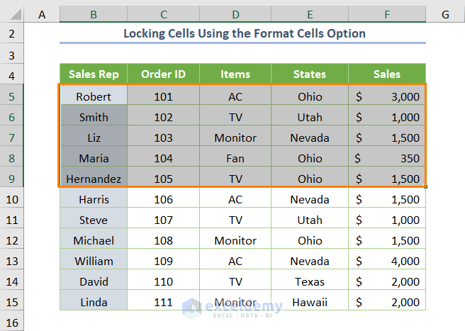
Afterward, open the Format Cells again (by pressing Ctrl + 1). And check the box before the Locked option.

Right now, your selected cells are locked and you need to turn on the protection of the sheet.
Step 03: Activating the Protection of Sheet
So, click on Protect Sheet in the Protect ribbon from the Review tab.
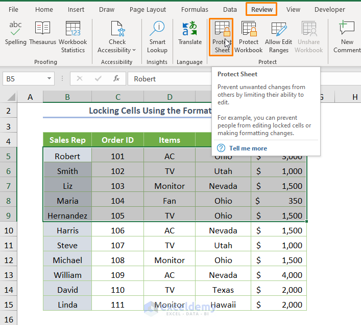
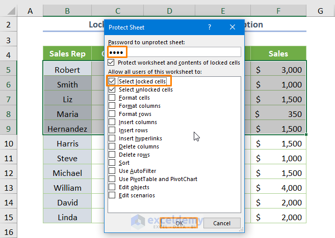
Immediately, you’ll see the following dialog box namely Protect Sheet.
Here, you need to input the password and press OK.
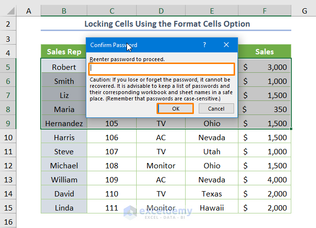
Again, you have to reenter your password as shown in the below screenshot.
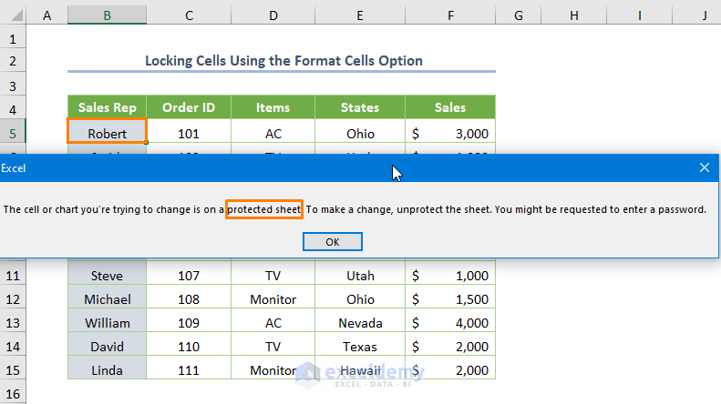
Subsequently, your selected cells are locked and protected. For example, if you click on the B5 cell to change or edit, you’ll get an error message which depicts your sheet is “a protected sheet” and you need to enter a password to edit.
Read More: How to Protect Excel Cells with Formulas
2. Adding a Button from Quick Access Toolbar
Furthermore, you might add the Lock Cell command in the Quick Access Toolbar (QAT) instead of using the Format Cells option.
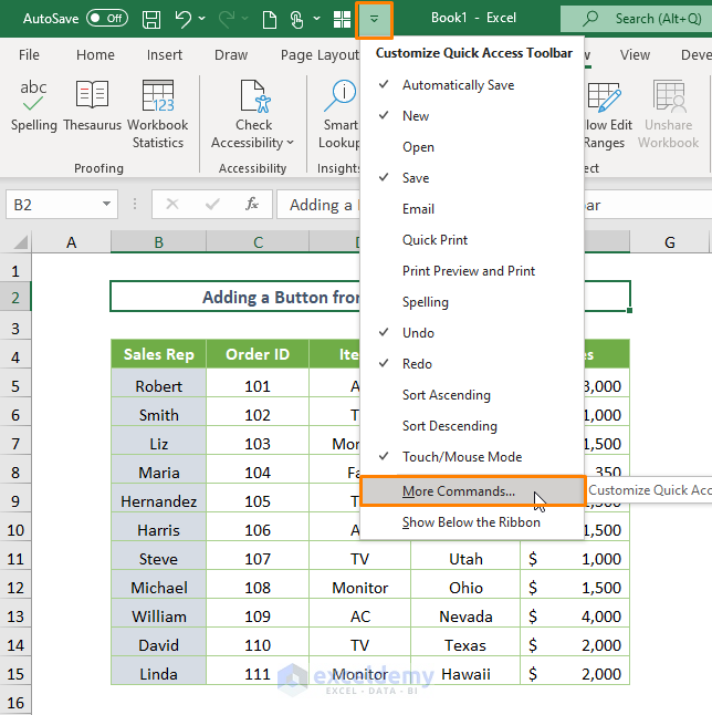
For adding the command, click on the icon of Customize Quick Access Toolbar and choose More Commands.
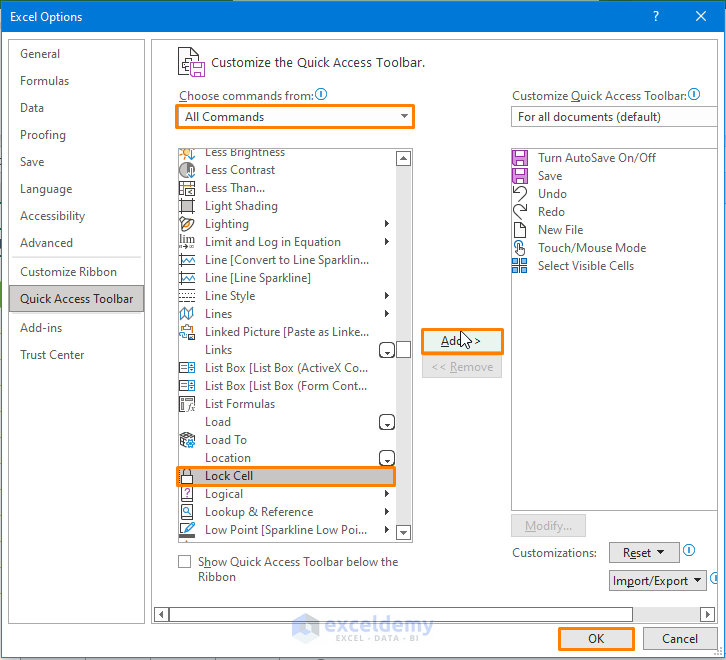
Then, choose All Commands from the drop-down list of the Choose commands from option.
Besides, select the Lock Cell option as shown in the following picture and click on the Add option. Finally, press OK.
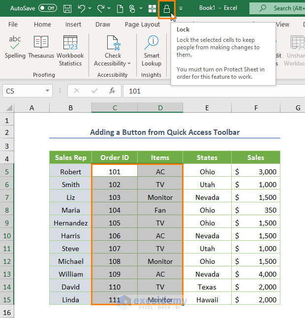
Within a short time, you’ll see an icon of the Lock Cell as shown in the following screenshot.
After removing the default “locked” option, select the multiple cells (e.g. C5:D15 cell range). Now, just click on the Lock Cell command from the Quick Access Toolbar.
Now, your selected cells are locked and you have to do the same task as discussed in the first method (step 3) to turn on the protection of the sheet.
Read More: How to Protect Excel Cells with Password
3. Locking Cells Having Formulas
More importantly, if you may require to lock certain multiple cells that have formulas, you might do that using this method.
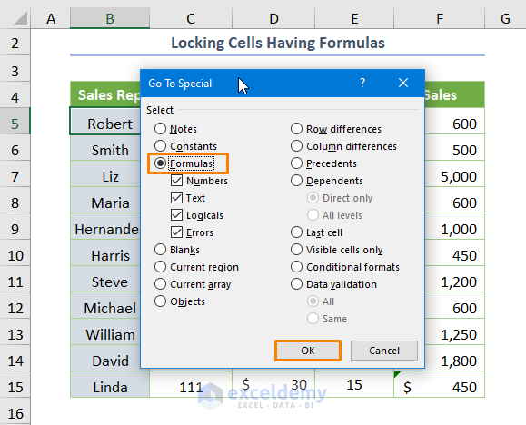
To find the cell having formulas, you may use the Go To Special option from the Find & Select option in the Home tab.
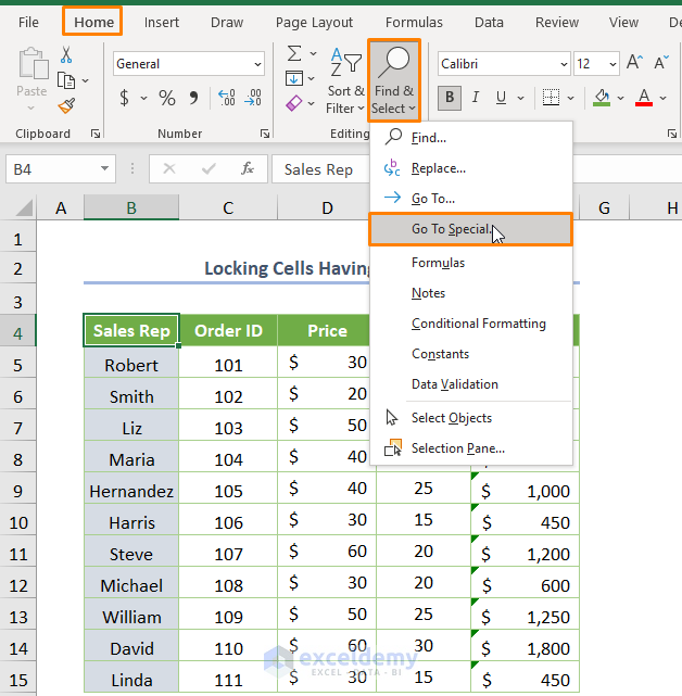
Then, check the circle before the Formulas option and press OK.
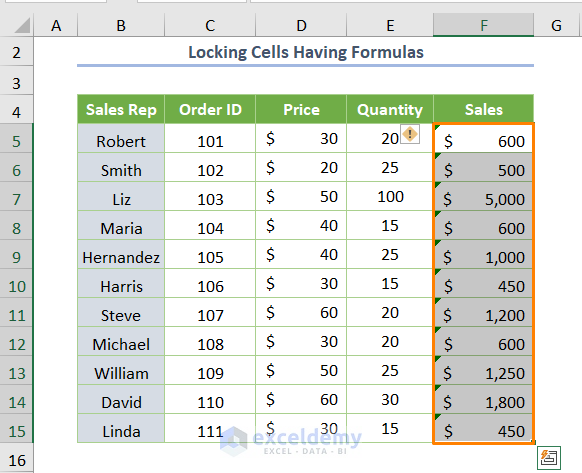
Shortly, you’ll get the cells having formulas (F5:F15 cell range).
Now, using the Format Cells discussed in the first method or Lock Cell command discussed in the second method, you may lock the specific cells. After that, you need to activate the protection of the sheet (step 3 of the first method).
Read More: How to Protect Excel Cells from Being Edited
4. Using VBA Code
In addition, if you are accustomed to using the VBA code, you might utilize the VBA to lock cells.
For example, you are able to lock the cell range B5:F8 in the dataset using the Macro.
Before doing that you have to create a module in the following way.
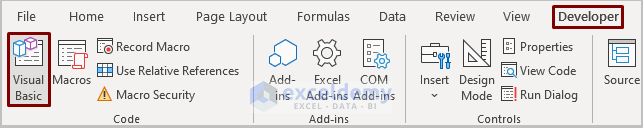
➤ Firstly, open a module by clicking the Developer tab > Visual Basic.
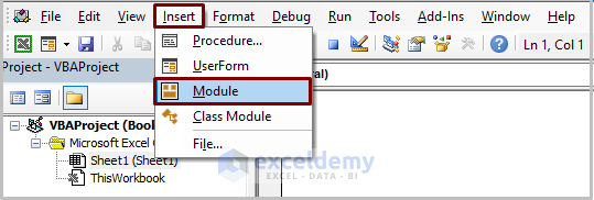
➤ Secondly, go to Insert > Module.
Now, just copy the following code into the newly created module.
Sub Locking_Protecting_MultipleCells()
Dim LPassword As String
Range("B5:F8").Select
Selection.Locked = True
LPassword = InputBox("Enter the Password to Protect")
ActiveSheet.Protect Password:=LPassword
End Sub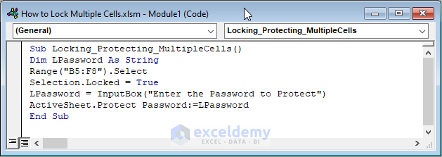
In the above code, we declared LPassword as a String type. Then, we select the cells using the Range.Select method. Thereafter, we used the Locked property as True to lock the cell range. Moreover, we assigned the InputBox to enter a password. Lastly, we utilized the Protect Password method to turn on the protection of the active sheet.
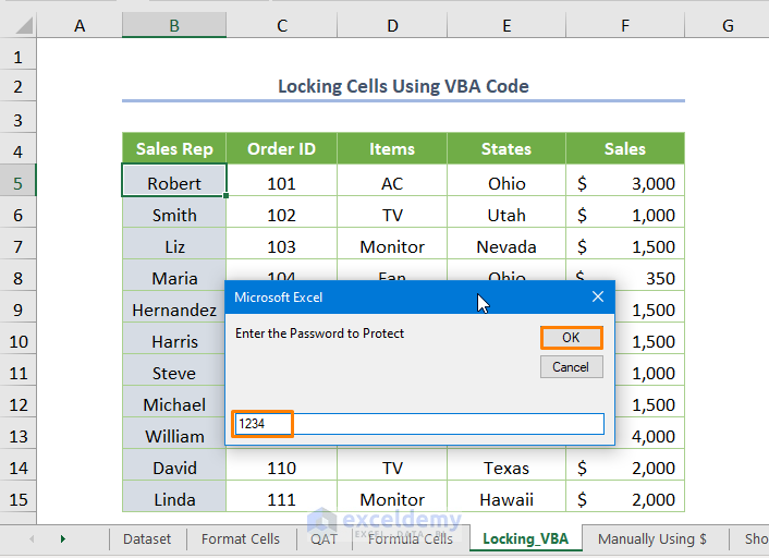
Next, when you run the code (the keyboard shortcut is F5 or Fn + F5), you’ll get a dialog box where you have to enter the password.
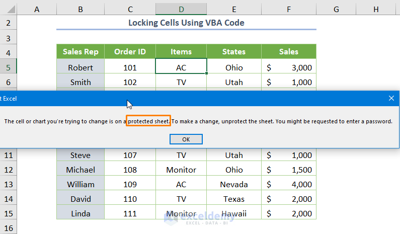
When you enter the password, immediately the selected cells are locked. If you want to check whether the cell is locked or not, just select a cell (e.g. D5 cell) and try to edit. Shortly, you’ll see an error message as depicted in the following screenshot.
How to Lock Multiple Cells with Dollar Sign ($): 2 Methods
1. Manually Locking Multiple Cells
Sometimes, we need to fix some specific cells to copy the whole formula for the below cells.
Assuming that you want to find the sales of some specific order Id using the VLOOKUP function.
=VLOOKUP(G5,B5:E15,4,FALSE)
Here, G5 is the lookup value, B5:E15 is the table array (cell range), 4 is the column index as the sales is located column no. 4 from the ‘Order ID’ column, and lastly FALSE is for exact matching.
Then, you have to insert the Dollar sign ($) within the table array manually. So, the absolute reference will be look like $B$5:$E$15 and the whole formula will be-
=VLOOKUP(G5,$B$5:$E$15,4,FALSE)
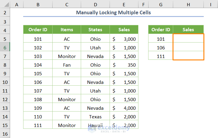
After pressing Enter, you’ll get the output as $3000 for 101 Order ID.
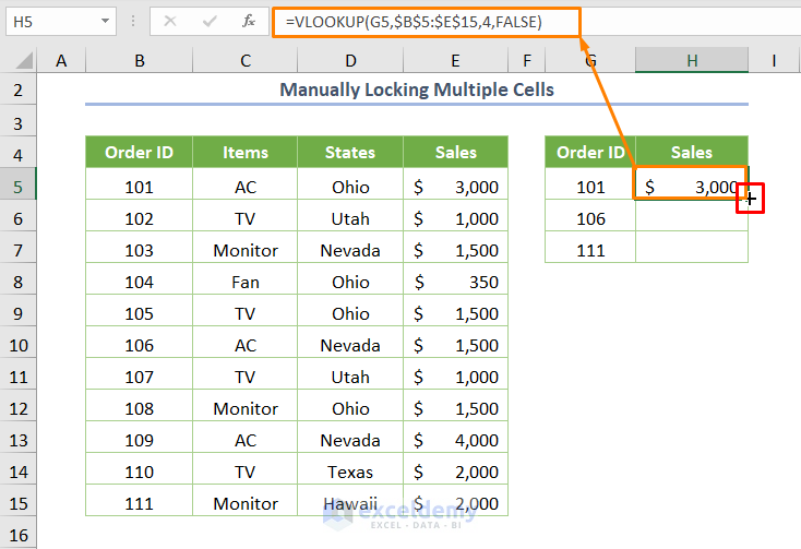
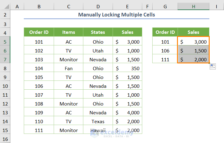
Furthermore, if you use the Fill Handle Tool (just drag down the plus sign in the above image), you’ll get the following output for other order Id.
Read More: How to Lock Cell Value Once Calculated in Excel
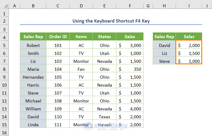
2. Using the Keyboard Shortcut F4 Key
Moreover, you may accomplish the same task (lock cells for using as the absolute references) utilizing the keyboard shortcut key (F4 key).
For using the shortcut key, go on the formula and select the cell range that you want to use the absolute references (e.g. B5:F15). And just press the F4 key keeping the cursor over the selected cell range.
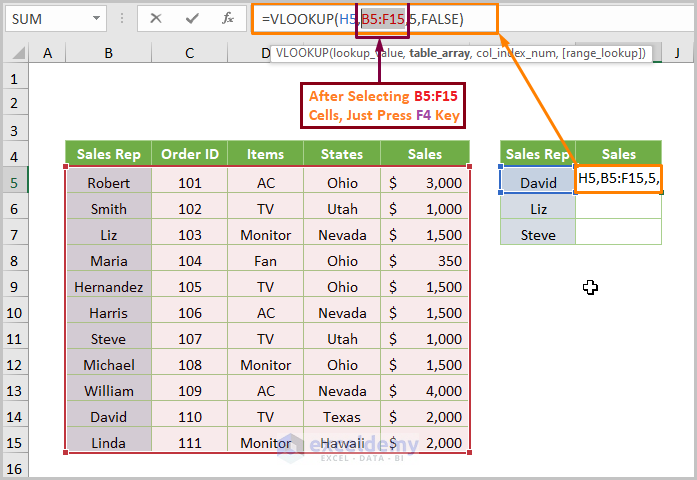
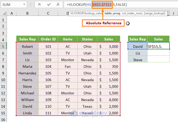
Automatically, you’ll see the $ sign within the cell range as shown in the below screenshot. So the formula will be-
=VLOOKUP(H5,$B$5:$F$15,5,FALSE)
If you press Enter and use the Fill Handle Tool, you’ll get the number of sales for a specified Sales Rep.
To use the shortcut key effectively in different situations, just have a look at the following table.
| Shortcut | Cell Reference | Description |
|---|---|---|
| Press F4 key | Multiple Cells | Allows changing neither the column nor the row. |
| Press the F4 key twice | Row Reference | Allows changing the column reference but the row reference is fixed. |
| Press the F4 key thrice | Column Reference | Allows changing the row reference but the column reference is fixed. |
Read More: How to Lock a Cell in Excel Formula
Things to Remember
- You should keep in mind that you have to remove the default ‘locked’ option for locking specific cells.
- If the F4 key doesn’t work on your pc, you may press Fn + F4 key.
Download Practice Workbook
Conclusion
This is how you may lock multiple cells in Excel using the discussed methods. We strongly believe this session will articulate your Excel journey. Anyway, if you have any queries or recommendations, please share them in the comments section.
Related Articles
- How to Protect Excel Cells from Deletion
- Protect Excel Cells But Allow Data Entry
- How to Protect Cells Without Protecting Sheet in Excel
- How to Lock Certain Cells in Excel
- How to Unlock Cells without Password in Excel
<< Go Back to Protect Excel Cells | Excel Protect | Learn Excel
Get FREE Advanced Excel Exercises with Solutions!
