The loan amortization schedule shows remaining debts along with paid principal and interest. Sometimes a moratorium period is given to borrowers under difficult circumstances. If a grace period is also given, the time period will increase. Otherwise, the EMI will change during the payoff to adjust the remaining balance.
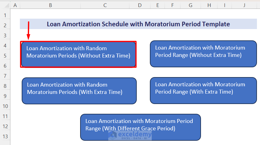
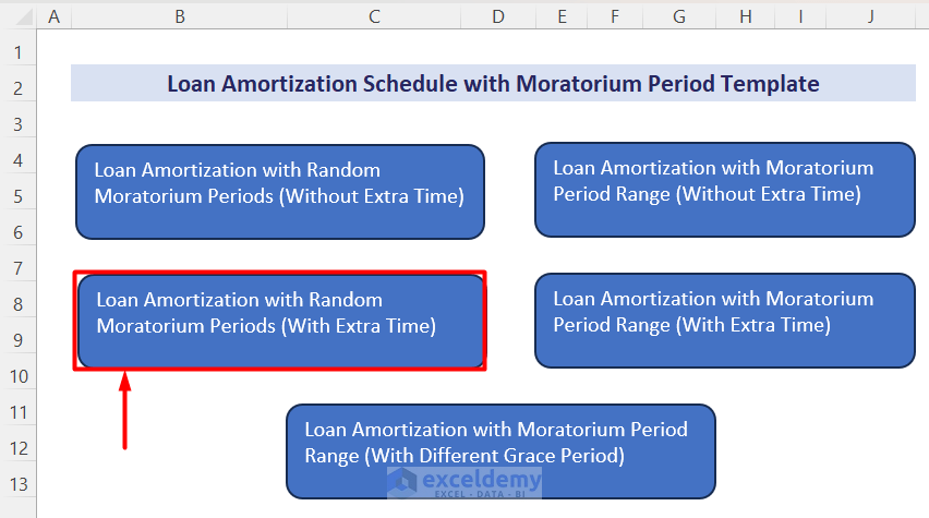
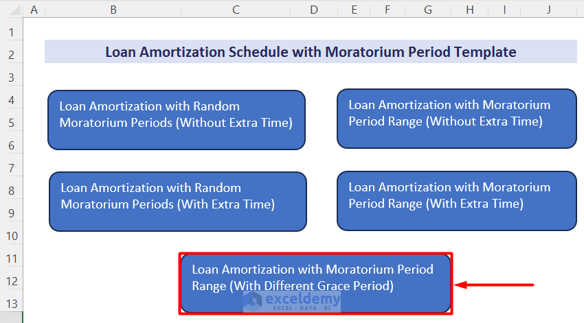
The free downloadable Excel template includes different grace periods, no grace periods, random moratorium selection, and moratorium period range.
Click to Enlarge the Image
Download Excel Templates
Download EXCEL (.XLSX)For: Excel 2007 or later
License: Private Use
What Is an Amortization Schedule?
The amortization schedule is a loan repayment schedule showing all values of payments, interest paid, principal paid, and remaining balance after each payment. Depending on loan amount and tenures, payment per installment is calculated, and a comparison of principal, interest, and remaining balance can be made.
What is the Moratorium Period and Grace Period?
Moratorium Period: The moratorium period is the period when the borrower is not obliged to pay regular payments. He will not be fined or charged extra. However, the regular interest payables will be added to his remaining loan balance.
Grace Period: According to Investopedia, the grace period is a fixed length of time that is given to borrowers after the due date to pay their loans without penalty.
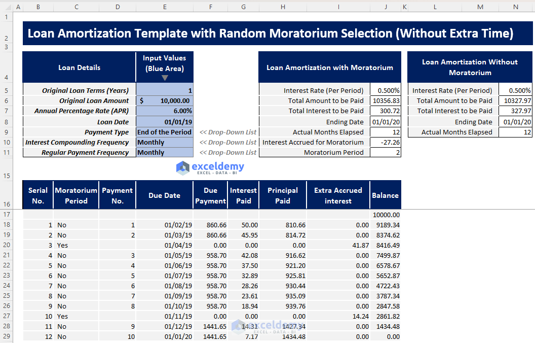
Template 1 – Loan Amortization Schedule with a Random Moratorium Period Selection (Without Extra Time)
Click to Enlarge the Image
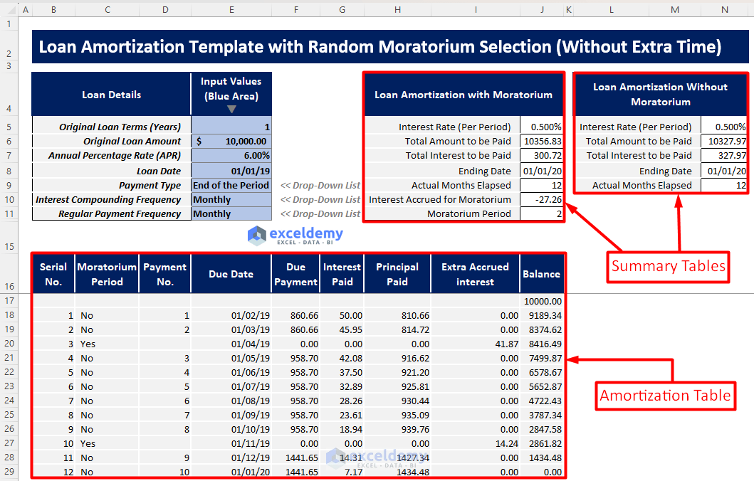
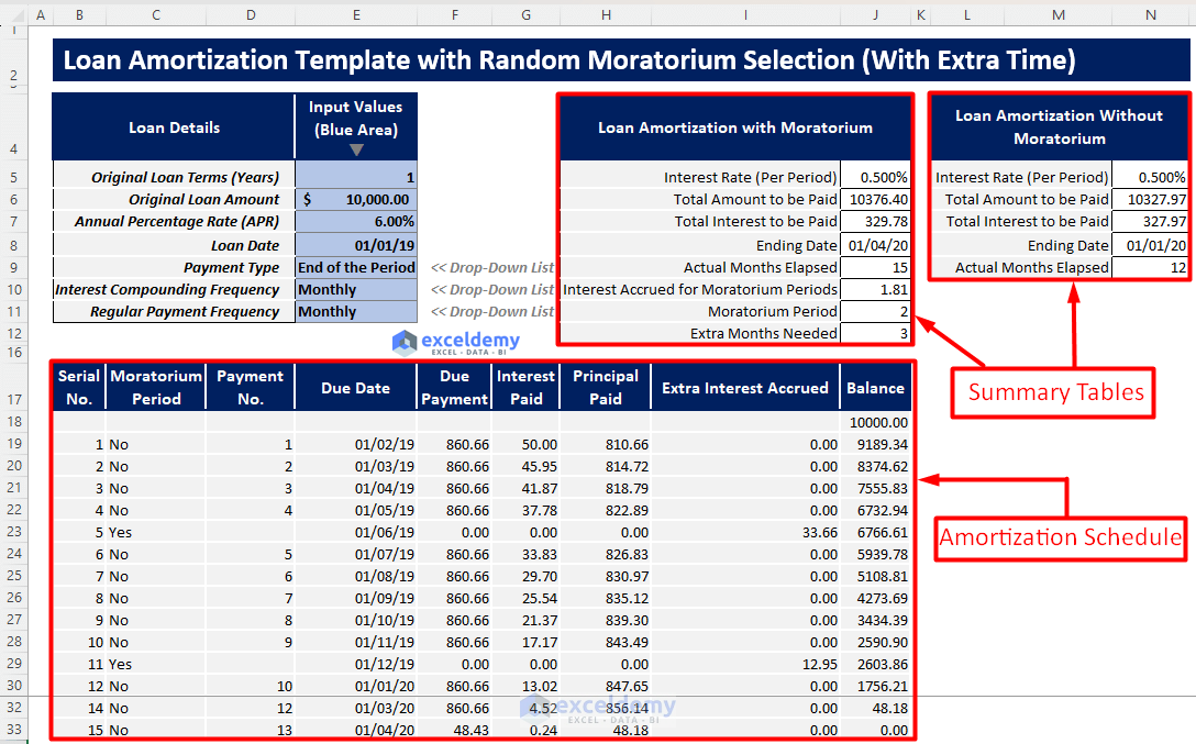
In this template, you will find a revised amortization schedule. You can select your moratorium periods with a Yes-No dropdown. There is no grace period. So, your EMI will increase.
How to Use This Template
Instructions:
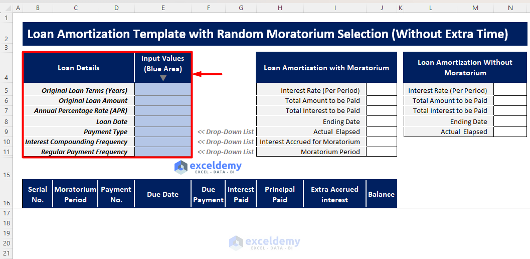
- Open the Excel file and go to the “Loan Amortization with Random Moratorium Periods (Without Extra Time)” template.
- you will find the input area in a blue-shaded fill.
- Find the names of the parameters in Loan Details. Enter values in the blue area and choose your options from the drop-down lists.
Click to Enlarge the Image
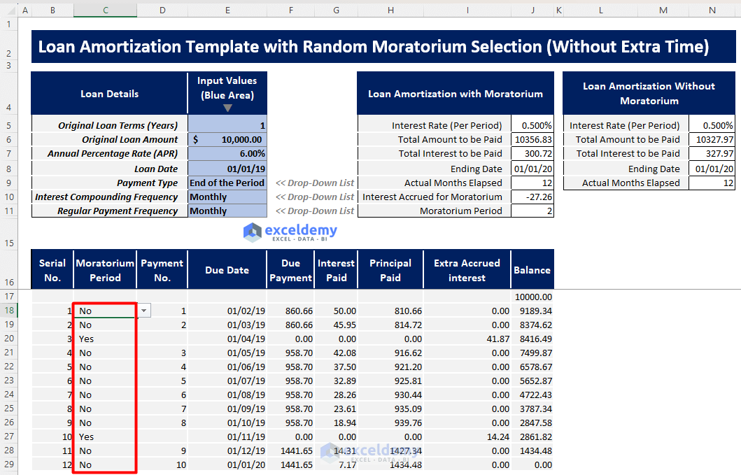
- Further calculations will automatically be done and you will get your amortization schedule. You can select a period of amortization as a Moratorium period.
Click to Enlarge the Image
- According to the input values and chosen moratorium periods, the EMI will always change to adjust your loan balance.
- In this case, no grace period is given. So the ending date of the loan will not change.
You will get a summary of the Amortization table with and without moratorium periods. You will be able to compare the values.
Click to Enlarge the Image
Read More: Loan Amortization Schedule with Variable Interest Rate in Excel
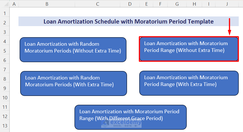
Template 2 – Loan Amortization Schedule with a Moratorium Period Range (Without Extra Time)
Click to Enlarge the Image
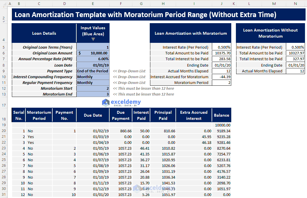
In this template, you will find your revised amortization table with a selected moratorium period range. Choose the moratorium range. It is assumed that there is no grace period. So, EMI will change to adjust the loan balance.
How to Use This Template
Instructions:
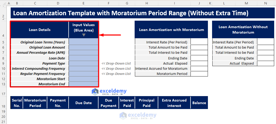
- Open the Excel file and go to the “Loan Amortization with Moratorium Period Range (Without Extra Time)” template.
- Enter your values in the blue shaded area in Input Values.
Click to Enlarge the Image
You will get the revised amortization schedule and two summary tables to compare loan amortization with and without moratorium periods.
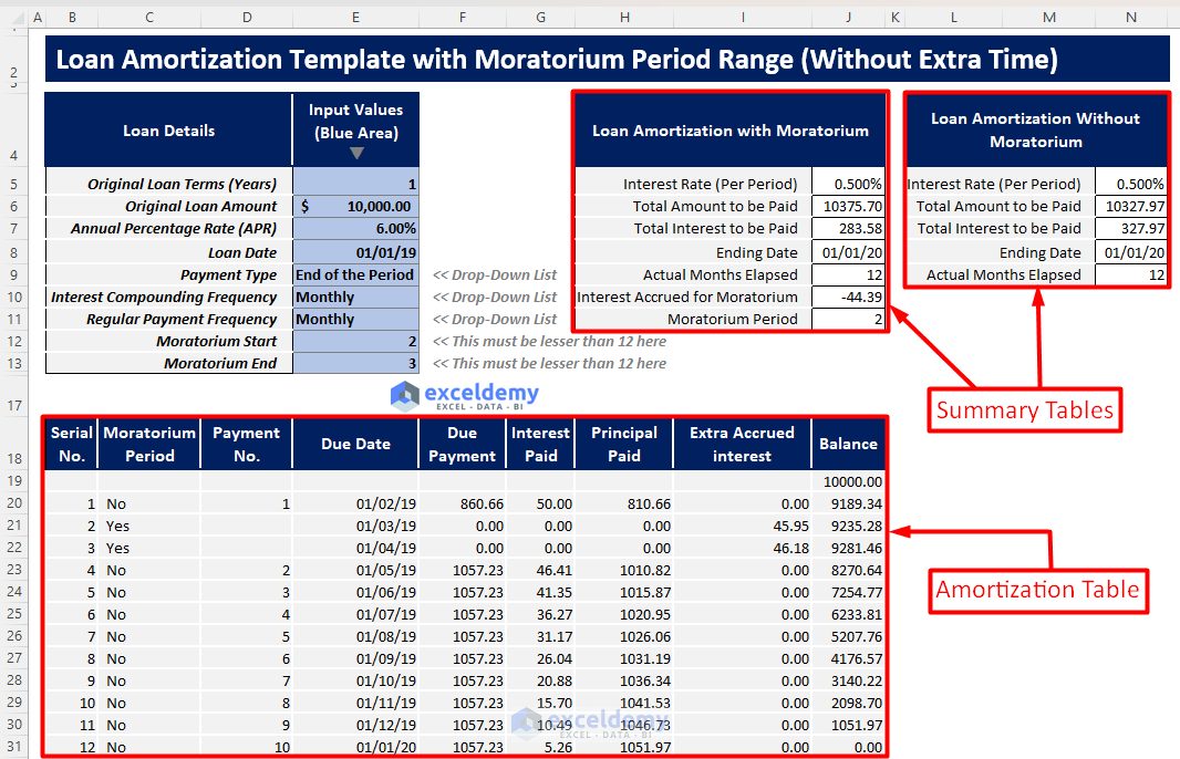
Click to Enlarge the Image
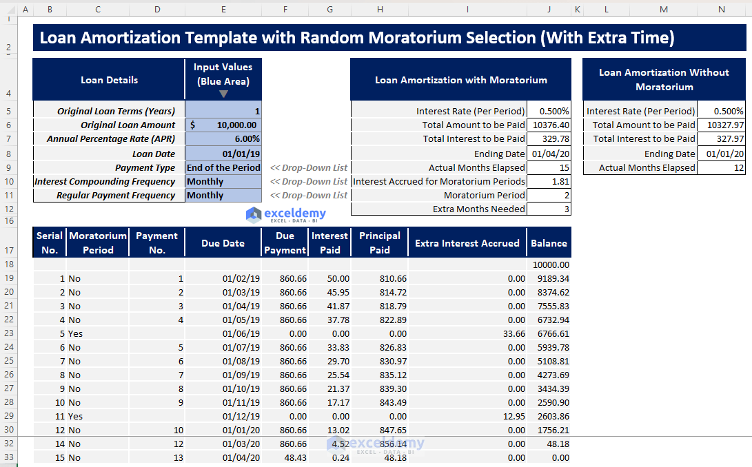
Template 3 – Loan Amortization Schedule with a Random Moratorium Period Selection (with Extra Time)
Click to Enlarge the Image
In this template, you will get your amortization schedule with moratorium and grace periods. You can select moratorium periods in the Yes-No dropdown. The EMI will remain the same throughout the pay. However, the ending date of loan repayment will change depending on the moratorium periods.
How to Use This Template
Instructions:
- Download the free template and click “Loan Amortization with Random Moratorium Periods (With Extra Time)”.
- Enter values in the blue shaded area according to the loan details.
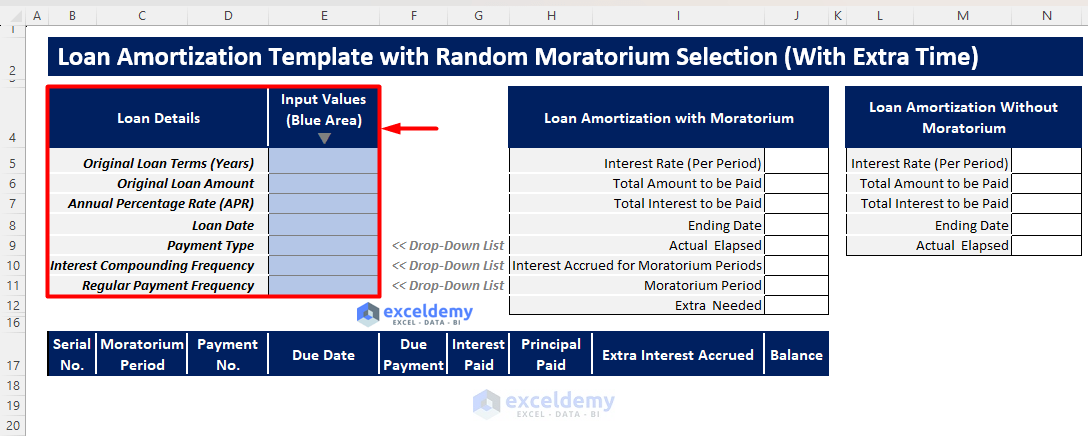
Click to Enlarge the Image
- Select moratorium periods as Yes or No in the Moratorium Period column.

Click to Enlarge the Image
You will get a completed and revised amortization schedule with two summary tables containing the results of amortization with and without moratorium periods.
Click to Enlarge the Image
Read More: Excel Monthly Amortization Schedule
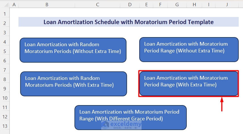
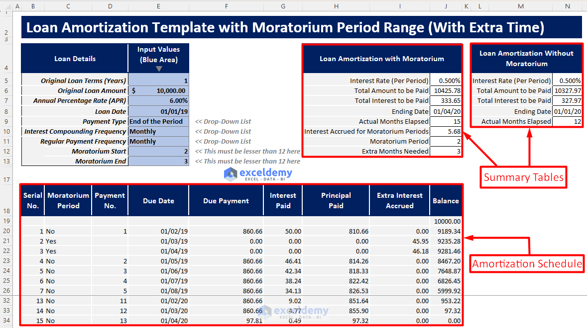
Template 4: Loan Amortization Schedule with a Moratorium Period Range (with Extra Time)
Click to Enlarge the Image
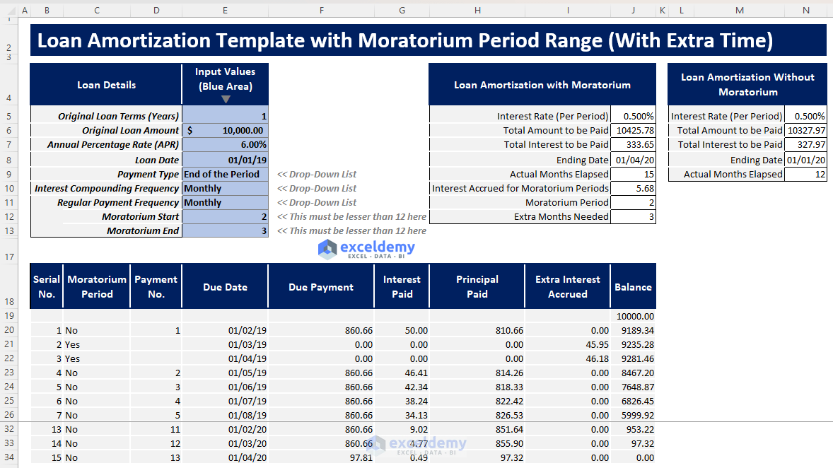
In this template, you will find your revised Amortization schedule with a moratorium period range and grace periods. You can select moratorium periods as ranges. This template is designed for allowed grace periods. EMI will not change over the periods, but the ending period will vary according to the chosen moratorium periods.
How to Use This Template
Instructions:
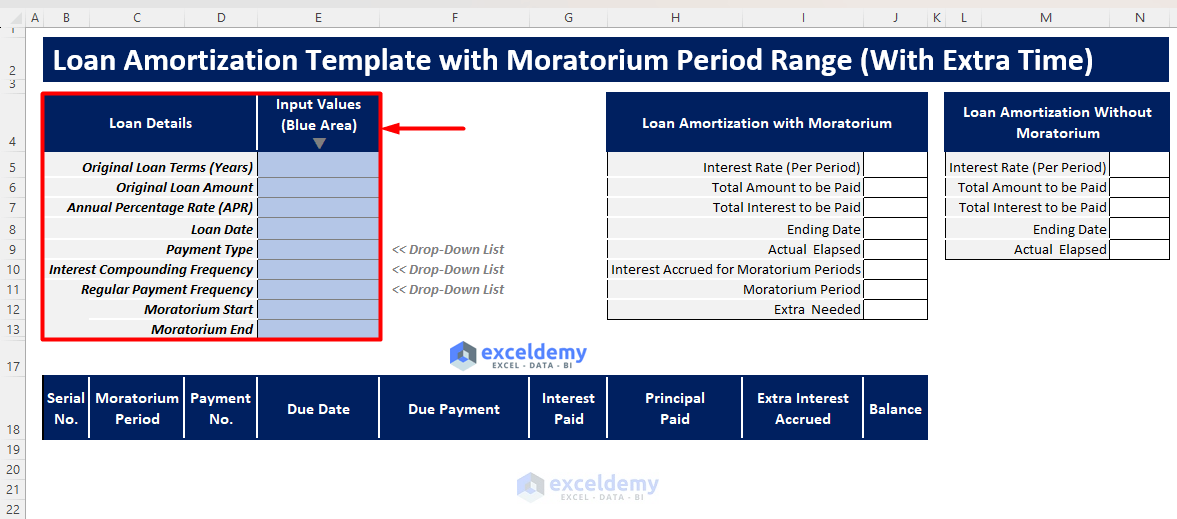
- Open the Excel file and click “Loan Amortization with Moratorium Period Range (With Extra Time)”.
- Enter values in the blue shaded area, according to Loan Details.
Click to Enlarge the Image
You will find your revised Amortization table and two summary tables to compare the amortization with and without moratorium periods.
Click Here to Enlarge the Image
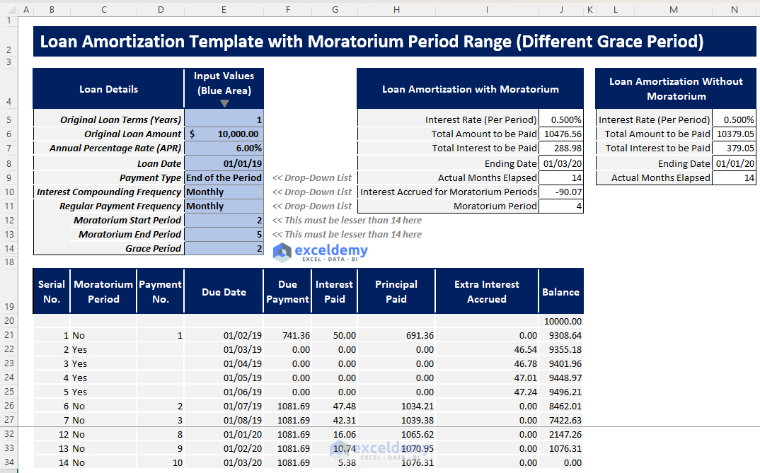
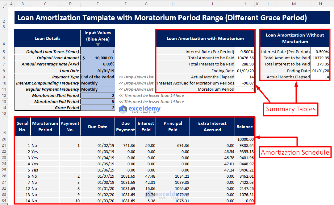
Template 5: Loan Amortization Schedule with a Moratorium Period Range (with Different Grace Periods)
Click Here to Enlarge the Image
In this template, you will find your revised amortization table with different moratorium and grace periods. The ending date will changedepending on the grace period. The EMI may change too according to the moratorium periods.
How to Use This Template
Instructions:
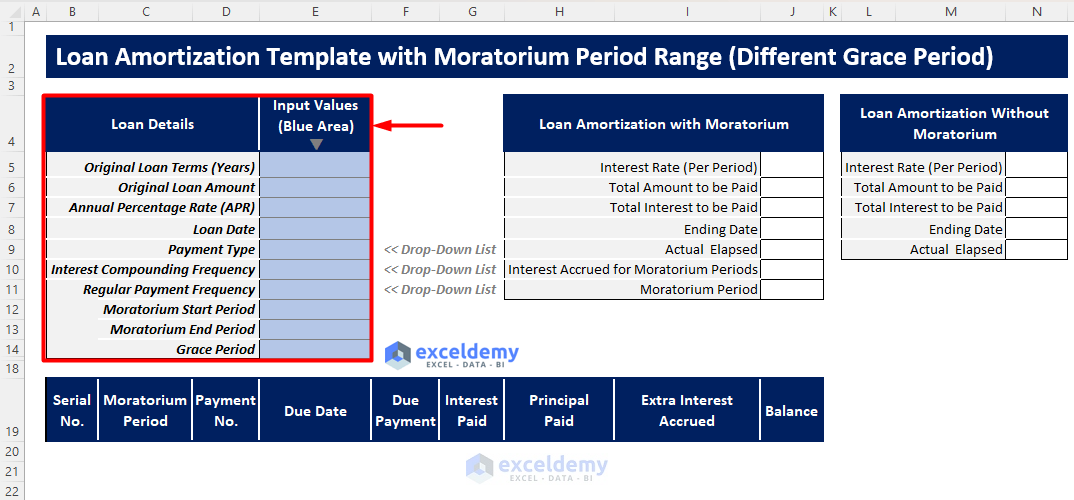
- Open the Excel file and click “Loan Amortization with Moratorium Period Range (With Different Grace Period)”.
- Enter values in the blue shaded area in Input Values according to the loan parameters.
Click to Enlarge the Image
You will get your amortization schedule and two summary tables to compare loan amortization with and without the moratorium.
Click Here to Enlarge the Image
Loan Amortization with Moratorium Tips
- Enter the Annual Percentage Rate directly in Input Values. Choose the interest compounding frequency and payment frequency in the dropdown. The interest rate will automatically be calculated.
- In the random moratorium selection templates, choose yes if the following period is the moratorium period. Otherwise, choose No.
- Enter Moratorium Start Period and Moratorium End Period values as less than the total number of initial periods.
- Choose Payment Type as Beginning of the Period if you pay your EMI at the beginning of the period, and choose End of the Period if you pay your EMI at the end of the period.
Related Articles
- EIDL Loan Amortization Schedule Excel
- Excel Actual/360 Amortization Calculator Template
- Excel 30 Year Amortization Schedule Template
- Excel Weekly Amortization Schedule
- Excel Quarterly Amortization Schedule
<< Go Back to Amortization Schedule | Finance Template | Excel Templates
Get FREE Advanced Excel Exercises with Solutions!

kindly give the calculation of moratorium period with PV formula for loan amortisation.
Very helpful.
Would you please provide me a soft copy of the same to my email address.
Regards
Hello Mf Sohel Rana,
Thanks for your feedback and appreciation. Download the Template from here: Loan Amortization Schedule in Excel with Moratorium Period [Free Download]
Keep exploring Excel with ExcelDemy!
Regards,
ExcelDemy