The VBA VLookup Function and the Named Range
Summary of the VBA VLookup Function
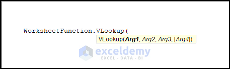
The VBA VLookup function finds a specified value from the first column of a defined table array and returns a value from another column of the same table array.
Syntax
WorksheetFunction.VLookup(Arg1, Arg2, Arg3, [Arg4])
the expression indicates a variable that refers to a Worksheet Function object.
Arguments
| Arguments | Required/Optional | Explanation |
|---|---|---|
| Arg1 | Required | the value that will be searched in the first column of the lookup_array. |
| Arg2 | Required | the range of the cells that contain data. |
| Arg3 | Required | the column number of the output column in the table_array. |
| Arg4 | Optional | denotes a logical value (TRUE/FALSE). TRUE searches for an approximate match of Arg1. FALSE searches for an exact match of Arg1. |
Named Range
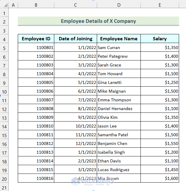
A named range is a collection of one or more cells that are given a name.
Consider the dataset below.
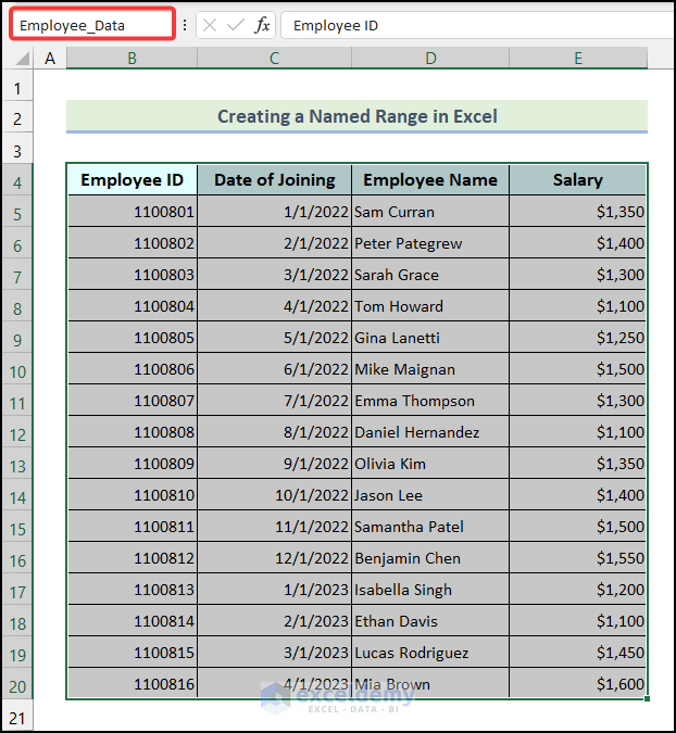
- Select the entire range >> click the Name Box.
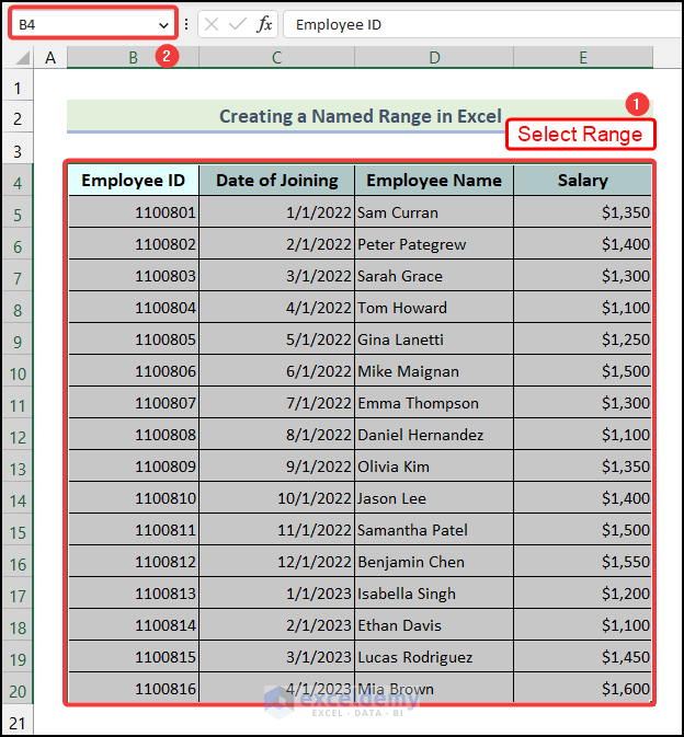
- Enter the name of the named range. Here, Employee_Data. Press ENTER.
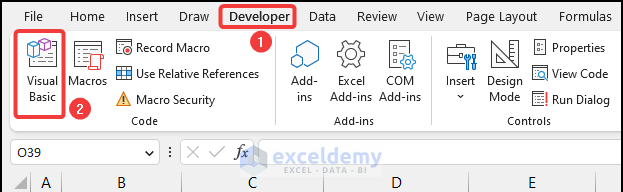
How to Launch the VBA Editor in Excel
- Go to the Developer tab >> click Visual Basic.
Note: If the Developer tab is not available, you can manually enable it.
- Go to the Insert tab >> Select Module.
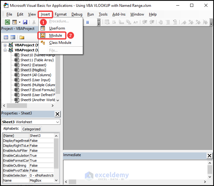
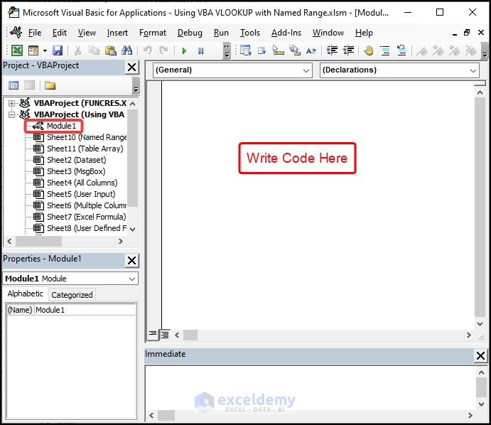
You can use your code in this Module.
Note: You can double-click any sheet name in the VB Editor and enter code there. However, codes that are entered in the sheets will only work in those sheets.Codes entered in a Module work on any sheet of the workbook.
Example 1 – Showing a Single Output from a specific Entry in the Named Range in a MsgBox
Steps:
- Create a Module >> Enter the following code >> click Save.
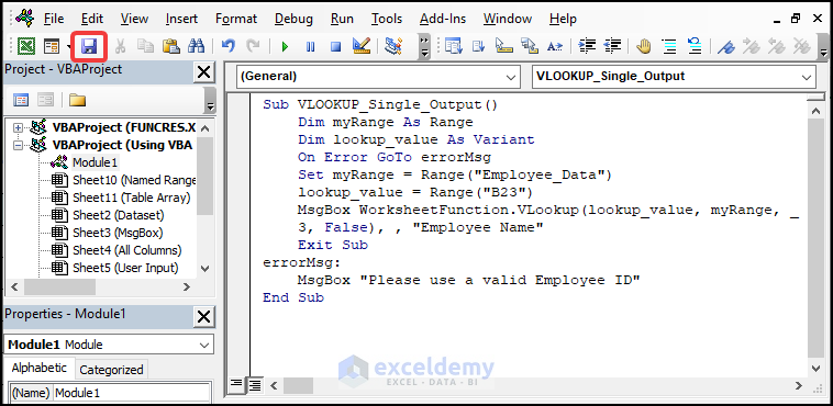
Sub VLOOKUP_Single_Output()
Dim myRange As Range
Dim lookup_value As Variant
On Error GoTo errorMsg
Set myRange = Range("Employee_Data")
lookup_value = Range("B23")
MsgBox WorksheetFunction.VLookup(lookup_value, myRange, _
3, False), , "Employee Name"
Exit Sub
errorMsg:
MsgBox "Please use a valid Employee ID"
End Sub
Code Breakdown
List of Variables Used
| Variable Name | Data Type |
|---|---|
| myRange | Range |
| lookup_value | Variant |
On Error GoTo errorMsg- If an error occurs, the On Error statement starts executing the code from the errorMsg block and skips all lines of codes in between.
Set myRange = Range("Employee_Data")
lookup_value = Range("B23")- The Set statement is used to define the data range (Employee_Data).
- B23 is assigned as lookup_value.
MsgBox WorksheetFunction.VLookup(lookup_value, myRange, _
3, False), , "Employee Name"
Exit Sub- The WorksheetFunction.VLookup method matches the first column of the named range with the lookup_value and returns values from the 3rd column of the named range if it finds an exact match.
- The MsgBox function shows the output in a MsgBox. Here, the title of the MsgBox is “Employee Name”.
- The code exits the sub-procedure.
errorMsg:
MsgBox "Please use a valid Employee ID"
End Sub- An error will occur if there is no match for Employee ID. A MsgBox will display “Please use a valid Employee ID” and the subprocedure ends.
- Press ALT + F11 and go back to the worksheet.
Running the Macro Using the Developer Tab:
- Enter a valid Employee ID in B23. Here, Employee ID 1100809.
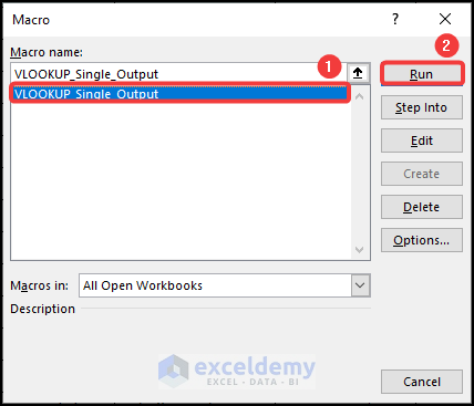
- Go to the Developer tab and choose Macros.
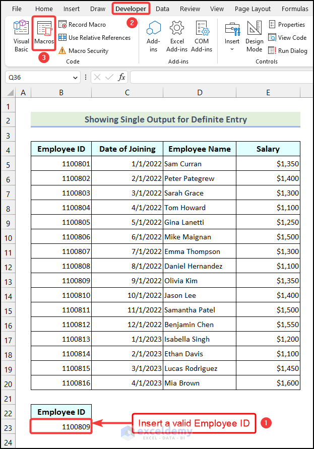
- In the Macro dialog box, select VLOOKUP_Single_Output and click Run.
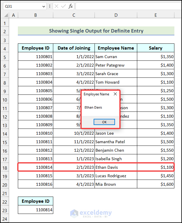
You will see the Employee Name for the Employee ID 1100809 displayed in a MsgBox:
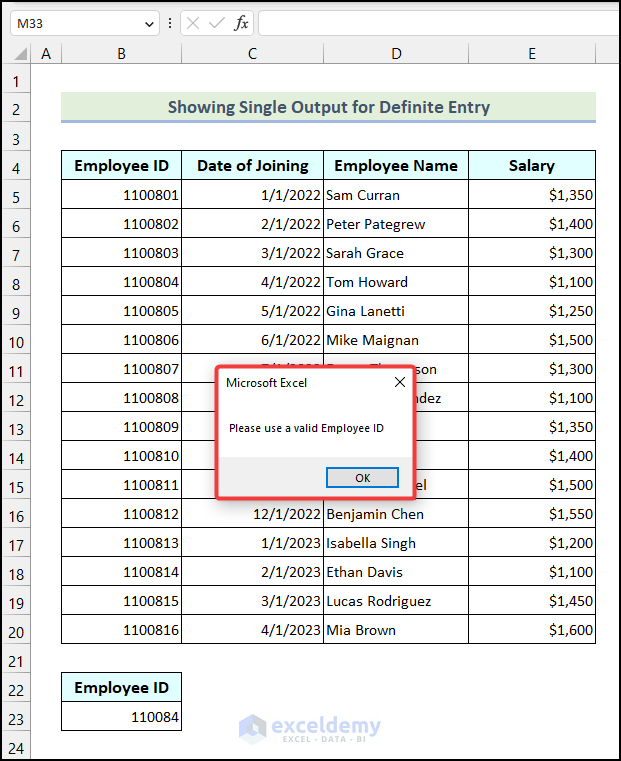
If you enter the wrong Employee ID in B23 and run the VBA code:
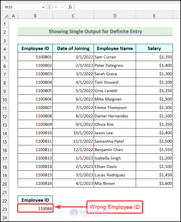
A MsgBox displays “Please use a Valid Employee ID”.
Read More: Excel VBA Vlookup with Multiple Criteria
Example 2 – VLookup Values from a Named Range using the User Input
Steps:
- Create a Module >> Use the following code >> click Save.
Sub VLOOKUP_Single_Output()
Dim myRange As Range
Dim lookup_value As Variant
On Error GoTo errorMsg
Set myRange = Range("Employee_Data")
lookup_value = Range("B23")
MsgBox WorksheetFunction.VLookup(lookup_value, myRange, _
3, False), , "Employee Name"
Exit Sub
errorMsg:
MsgBox "Please use a valid Employee ID"
End Sub
Code Breakdown
List of Variables Used
| Variable Name | Data Type |
|---|---|
| myRange | Range |
| lookup_value | Variant |
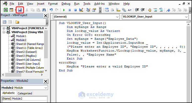
lookup_value = Int(Application.InputBox _
("Please enter an Employee ID", "Employee ID", , , , , , 8))- The Application.InputBox method takes the user and assigns it to the lookup_value variable.
- “Please enter an Employee ID” is the message that will be displayed in the InputBox. 8 indicates the Type parameter of the Application.InputBox method.
MsgBox WorksheetFunction.VLookup(lookup_value, myRange, 3, _
False), , "Employee Name"- A MsgBox is used to show the output after using the VBA VLookup function.
- Save the code.
- Press ALT + F11.
- Go back to the worksheet.
Running the Macro using a Keyboard Shortcut:
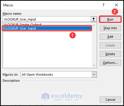
- To open the Macro dialog box, press ALT + F8.
- Select VLOOKUP_User_Input.
- Click Run.
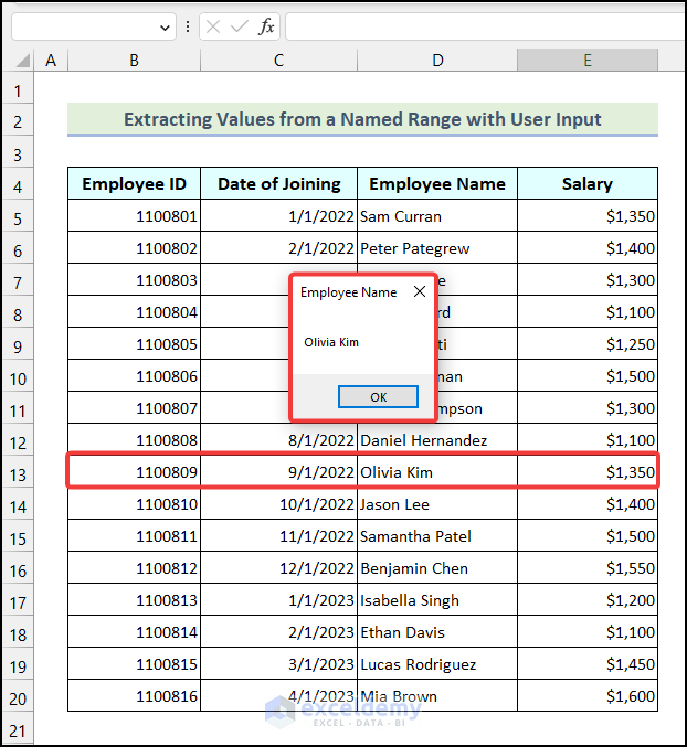
A dialog box named Employee ID will be displayed in your worksheet:
- Click the Employee ID dialog box >> choose any cell in the Employee ID column >> click OK.
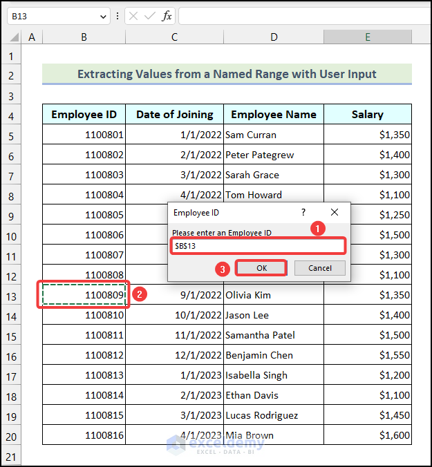
The Employee Name for the selected Employee ID will be displayed in an MSgBox.
Example 3 – Extracting All Columns Data for a specific Entry from a Named Range
Steps:
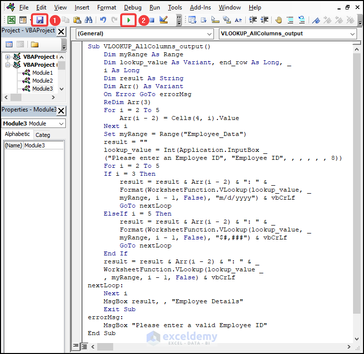
- Create a Module >> Enter the VBA code >> Click Save.
- Click Run Sub/Userform in the VB Editor window.
Sub VLOOKUP_Single_Output()
Dim myRange As Range
Dim lookup_value As Variant
On Error GoTo errorMsg
Set myRange = Range("Employee_Data")
lookup_value = Range("B23")
MsgBox WorksheetFunction.VLookup(lookup_value, myRange, _
3, False), , "Employee Name"
Exit Sub
errorMsg:
MsgBox "Please use a valid Employee ID"
End Sub
Code Breakdown
List of Variables Used
| Variable Name | Data Type |
|---|---|
| myRange | Range |
| lookup_value | Variant |
| end_row | Long |
| i | Long |
| result | String |
| Arr | Variant |
ReDim Arr(3)- the ReDim statement specifies the size of the array. Here, 3.
For i = 2 To 5
Arr(i - 2) = Cells(4, i).Value
Next j- A For Next loop stores column headers of row 4 in the array by looping through column B to column E.
For i = 2 To 5
If i = 3 Then
result = result & Arr(i - 2) & ": " & _
Format(WorksheetFunction.VLookup(lookup_value, _
myRange, i - 1, False), "m/d/yyyy") & vbCrLf
GoTo nextLoop
ElseIf i = 5 Then
result = result & Arr(i - 2) & ": " & _
Format(WorksheetFunction.VLookup(lookup_value, _
myRange, i - 1, False), "$#,###") & vbCrLf
GoTo nextLoop
End If
result = result & Arr(i - 2) & ": " & _
WorksheetFunction.VLookup(lookup_value _
, myRange, i - 1, False) & vbCrLf
nextLoop:
Next i- The VBA If Statement checks whether the current column is column C. If it is column C, the WorksheetFunction.VLookup method will be used and format the output as a date.
- This output is concatenated with the column headers in row 4 and the vbCrLf constant of VBA is added to insert a line break. This is assigned to the result variable.
- The nextLoop block uses the GoTo statement. If the current column is column C, this part of the For Next loop will be executed.
- ElseIf statement checks whether the current column is column E. If it is column E, the output will be in currency format.
- If the current column is neither column B nor column E, no formatting is added.
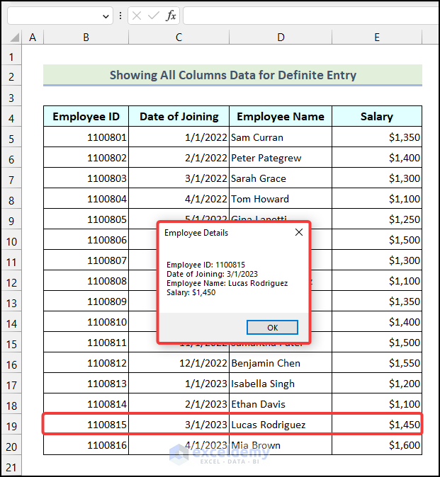
- Click the dialog box >> select any cell in the Employee ID column >> click OK.
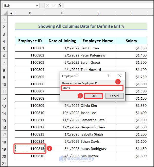
All data in all columns will be displayed in a MsgBox:
Read More: How to Use Excel VBA VLookup Within Loop
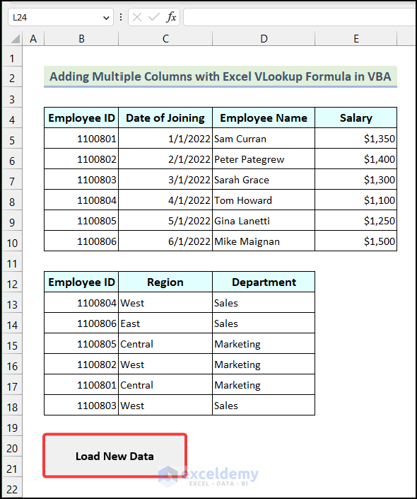
Example 4 – Adding Multiple Columns from Different Named Ranges with Matched Columns
4.1. Using the VLookup Result Only
Steps:
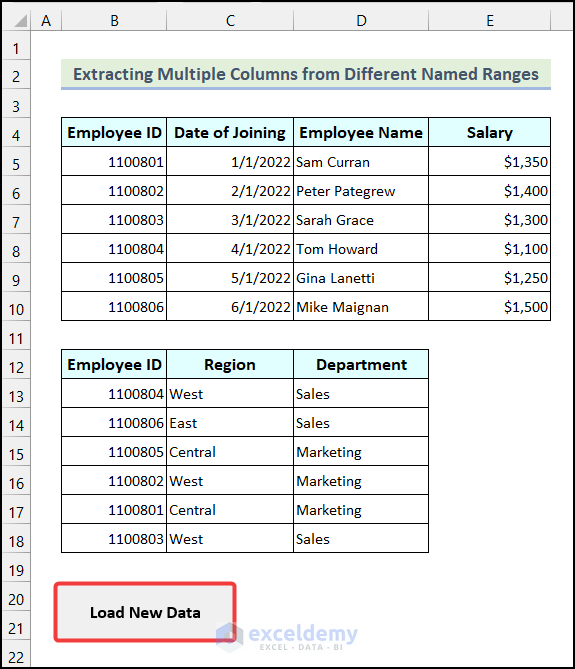
- Create a named range in B12:D18. Here, “New_Data”.
- Create a Module >> enter the VBA code >> click Save.
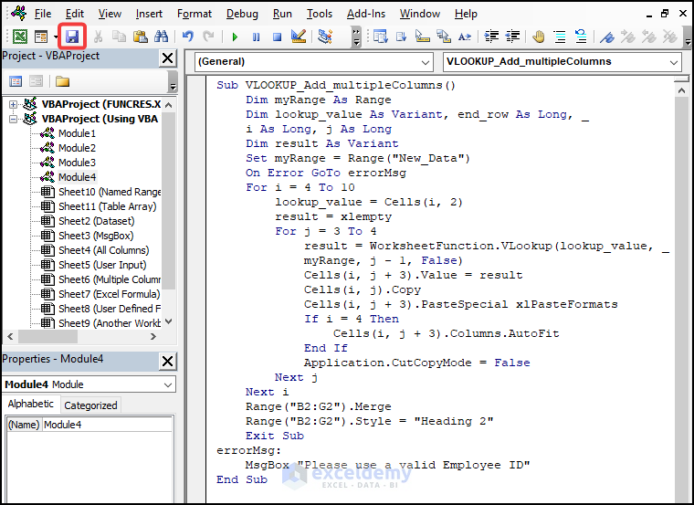
Sub VLOOKUP_Add_multipleColumns()
Dim myRange As Range
Dim lookup_value As Variant, end_row As Long, i As Long, j As Long
Dim result As Variant
Set myRange = Range("New_Data")
On Error GoTo errorMsg
For i = 4 To 10
lookup_value = Cells(i, 2)
result = xlempty
For j = 3 To 4
result = WorksheetFunction.VLookup(lookup_value, myRange, j - 1, False)
Cells(i, j + 3).Value = result
Cells(i, j).Copy
Cells(i, j + 3).PasteSpecial xlPasteFormats
If i = 4 Then
Cells(i, j + 3).Columns.AutoFit
End If
Application.CutCopyMode = False
Next j
Next i
Range("B2:G2").Merge
Range("B2:G2").Style = "Heading 2"
Exit Sub
errorMsg:
MsgBox "Please use a valid Employee ID"
End Sub
Code Breakdown
List of Variables Used
| Variable Name | Data Type |
|---|---|
| myRange | Range |
| lookup_value | Variant |
| end_row | Long |
| i | Long |
| j | Long |
| result | Variant |
For i = 4 To 10
lookup_value = Cells(i, 2)
result = xlempty
For j = 3 To 4
result = WorksheetFunction.VLookup(lookup_value, myRange, j - 1, False)
Cells(i, j + 3).Value = result
Cells(i, j).Copy
Cells(i, j + 3).PasteSpecial xlPasteFormats
If i = 4 Then
Cells(i, j + 3).Columns.AutoFit
End If
Application.CutCopyMode = False
Next j
Next i- The outer loop loops through the rows of the output range. Here, from row 4 to row 10. The inner For Next loop loops through the 2nd and 3rd columns of the “New_Data” range.
- The cells of column B in the output range are assigned as the lookup_value.
- A VLookup operation is used for each column using the index number “j-1,”, the lookup_value variable, and the range “myRange“. The “result” variable receives the lookup outcome as its value.
- The value of the result variable is assigned to cell(i,j+3) which refers to F4 in the worksheet.
- A cell from the current row is copied and the formatting is pasted in the cell where the value of the result variable is stored.
- An If statement checks whether the current row is row 4. If it is row 4, the column width is auto-fit using the Range.AutoFit method. The Application.CutCopyMode property is set to False.
Range("B2:G2").Merge
Range("B2:G2").Style = "Heading 2"
Exit Sub- Cells in B2:G2 are merged, using the Range.Merge method. The Cell Style of the merged range is specified to “Heading 2”. The code exits the sub-procedure.
Running Code by using a Button:
- Go to the Developer >> select Insert in Controls >> click Button (From Control).
- Draw the shape of the button as shown below.
- In the Assign Macro dialog box, select VLOOKUP_Add_multipleColumns.
- Click OK.
- Click the button to rename it. Here, “Load New Data”.
- Right-click the button.
In the Format Control dialog box:
- Choose a font in Font >> select Bold in Font Style >> define the font size >> click OK.
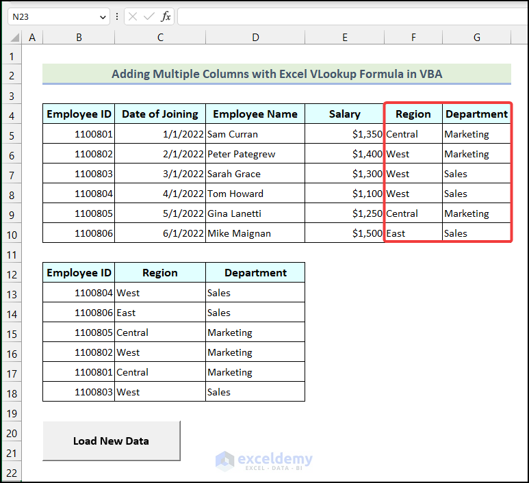
This is the output.
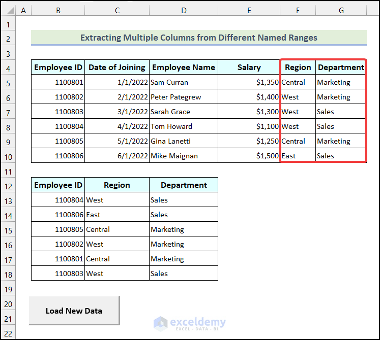
- Click the button to run the code.
The Region and Department columns in the named range “New_Data” are automatically added to the dataset.
4.2. Using the Worksheet Function in VBA
Steps:
- Create a Module >> enter the VBA code >> click Save.
Sub VLOOKUP_Add_multipleColumns()
Dim myRange As Range
Dim lookup_value As Variant, end_row As Long, i As Long, j As Long
Dim result As Variant
Set myRange = Range("New_Data")
On Error GoTo errorMsg
For i = 4 To 10
lookup_value = Cells(i, 2)
result = xlempty
For j = 3 To 4
result = WorksheetFunction.VLookup(lookup_value, myRange, j - 1, False)
Cells(i, j + 3).Value = result
Cells(i, j).Copy
Cells(i, j + 3).PasteSpecial xlPasteFormats
If i = 4 Then
Cells(i, j + 3).Columns.AutoFit
End If
Application.CutCopyMode = False
Next j
Next i
Range("B2:G2").Merge
Range("B2:G2").Style = "Heading 2"
Exit Sub
errorMsg:
MsgBox "Please use a valid Employee ID"
End Sub
Code Breakdown
List of Variables Used
| Variable Name | Data Type |
|---|---|
| myRange | Range |
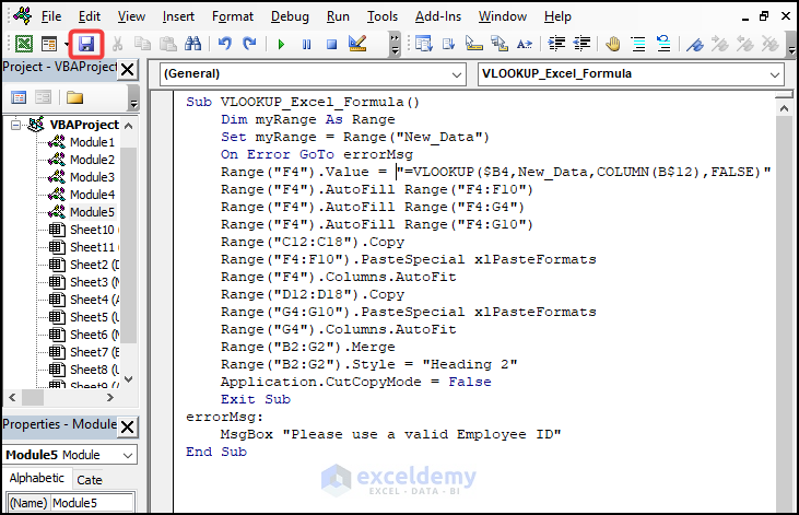
Range("F4").Value = "=VLOOKUP($B4,New_Data,COLUMN(B$12),FALSE)"
Range("F4").AutoFill Range("F4:F10")
Range("F4").AutoFill Range("F4:G4")
Range("F4").AutoFill Range("F4:G10")- The VLOOKUP function extracts values from a different named range (“New_Data) and the result is assigned to F4.
- The Range.AutoFill method copies this formula up to F10.
- The formula is copied horizontally to the next cell and and up to G10 using the Range.AutoFill method.
Range("C12:C18").Copy
Range("F4:F10").PasteSpecial xlPasteFormats
Range("F4").Columns.AutoFit
Range("D12:D18").Copy
Range("G4:G10").PasteSpecial xlPasteFormats
Range("G4").Columns.AutoFit- The formatting of the 2nd and 3rd columns in “New_Data” is copied and pasted in columns F and G, using the Range.PasteSpecial method. xlPasteFormats specifies that only the formatting should be pasted, not the cell content.
- The column width of column F and column G is autofit, using the Range.AutoFit method.
- Create a button and assign the VLOOKUP_Excel_Formula macro to the button by following the steps described in the previous method.
- Click the button to run the code.
The Region and the Department columns in the “New_Data” range are added:
Read More: Excel VBA to Vlookup Values for Multiple Matches
Example 5 – Creating a User-Defined Function to Apply the VBA VLookup Function with a Named Range
Steps:
- Create a Module and enter the VBA code >> click Save.
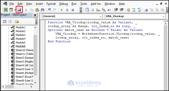
Function VBA_Vlookup(lookup_value As Variant, _
lookup_array As Range, col_index_no As Long, _
Optional match_case As Boolean = False) As Variant
    VBA_Vlookup = WorksheetFunction.VLookup(lookup_value, _
    lookup_array, col_index_no, match_case)
End Function
Code Breakdown
Function VBA_Vlookup(lookup_value As Variant, lookup_array As Range, col_index_no As Long, Optional match_case As Boolean = False) As Variant- The VBA_Vlookup function is created with the following arguments. The data type of the return value is set as Variant.
| Arguments | Required/Optional | Explanation |
|---|---|---|
| lookup_value | Required | the value to be found in the first column of the lookup_array range. |
| lookup_array | Required | the range of cells to search for the lookup_value and extract the output values. |
| col_index_no | Required | the column number in the lookup_array range to extract the output. |
| match_case | Optional | defines an exact match or an approximate match. |
VBA_Vlookup = WorksheetFunction.VLookup(lookup_value, lookup_array, col_index_no, match_case)- The WorksheetFunction.VLookup method performs the VLookup operation and assigns the output to the VBA_Vlookup function.
- The function ends.
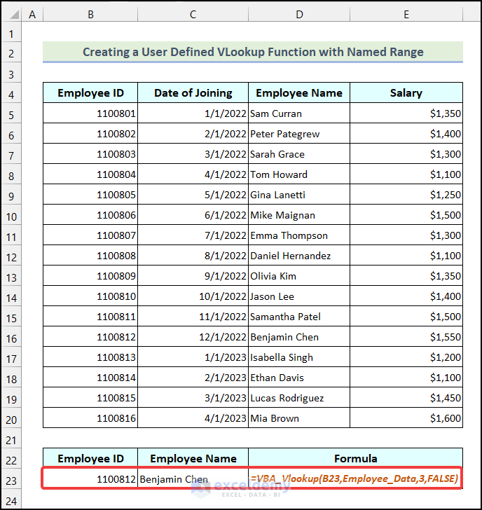
- Enter the following formula in C23.
- Press ENTER.
=VBA_Vlookup(B23,Employee_Data,3,FALSE)
B23 represents the Employee ID which is the lookup_value argument, Employee_Data is the named range defined as lookup_array argument, 3 is the number of columns in the lookup_array, and FALSE indicates an exact match.
You will get the Employee Name, according to the Employee ID.
How to Use the VBA VLookup Function with a Named Range in Another Workbook in Excel
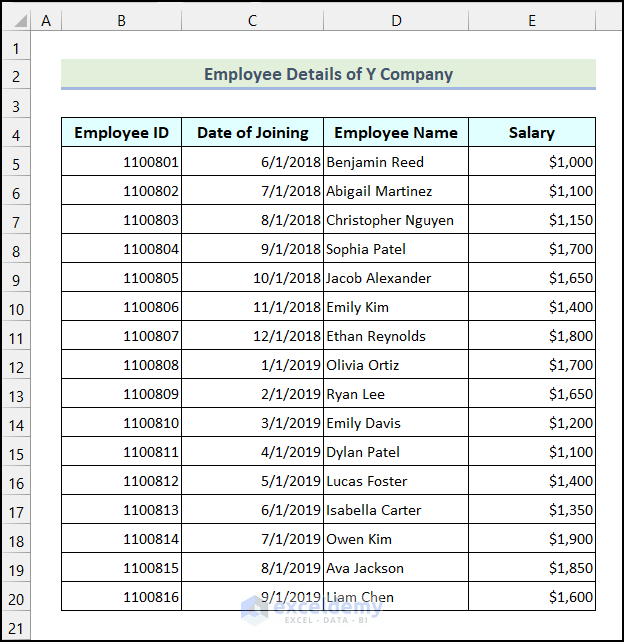
There are two Excel workbooks. “Sample Dataset” contains the following data range: B4:E20, named “Another_WB”.
Steps:
- Create a new Module in your original workbook (not in the “Sample Dataset” workbook) >>Enter the VBA code >> click Save.
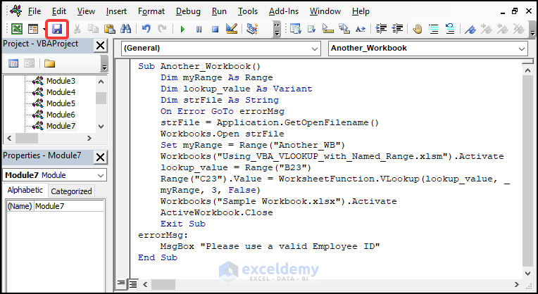
Sub Another_Workbook()
Dim myRange As Range
Dim lookup_value As Variant
Dim strFile As String
On Error GoTo errorMsg
strFile = Application.GetOpenFilename()
Workbooks.Open strFile
Set myRange = Range("Another_WB")
Workbooks("Using_VBA_VLOOKUP_with_Named_Range.xlsm").Activate
lookup_value = Range("B23")
Range("C23").Value = WorksheetFunction.VLookup(lookup_value, _
myRange, 3, False)
Workbooks("Sample Workbook.xlsx").Activate
ActiveWorkbook.Close
Exit Sub
errorMsg:
MsgBox "Please use a valid Employee ID"
End Sub
Code Breakdown
List of Variables Used
| Variable Name | Data Type |
|---|---|
| myRange | Range |
| lookup_value | Variant |
| strFile | String |
strFile = Application.GetOpenFilename()
Workbooks.Open strFile- The Application.GetOpenFilename method displays a dialog box, so that you can get the name of the file from which you need to extract data.
- The Workbooks.Open method opens that Excel file.
Workbooks("Using VBA VLookup with Named Range.xlsm").Activate
lookup_value = Range("B23")
Range("C23").Value =WorksheetFunction.VLookup(lookup_value, _ myRange, 3, False)- The initial workbook is activated using the Workbook.Activate method.
- The WorksheetFunction.VLookup method gets the data from another workbook and assigns the output to C23.
Workbooks("Sample Workbook.xlsx").Activate
ActiveWorkbook.Close
Exit Sub- The ActiveWorkbook.Close method closes the initial file.
- The code exits the sub-routine.
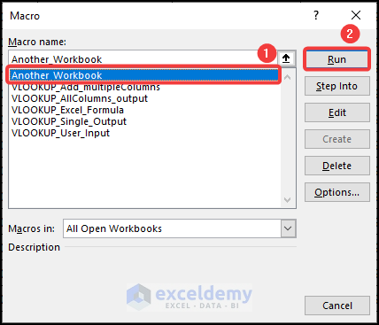
- Press ALT + F8 to open the Macro dialog box. Select Another_Workbook and click Run.
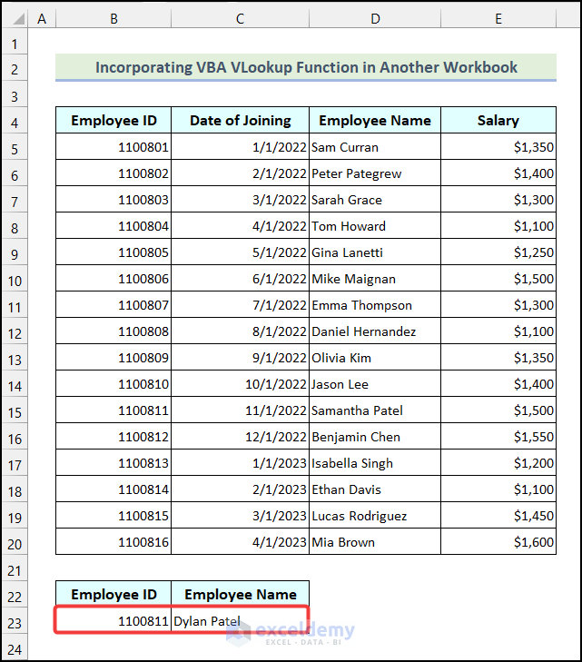
The code extracts the Employee Name from the “Sample Dataset” workbook:
How to Use the VBA VLookup Function with a Table Array in Excel
Steps:
- Create a blank Module >> Enter the VBA code >> Click Save.
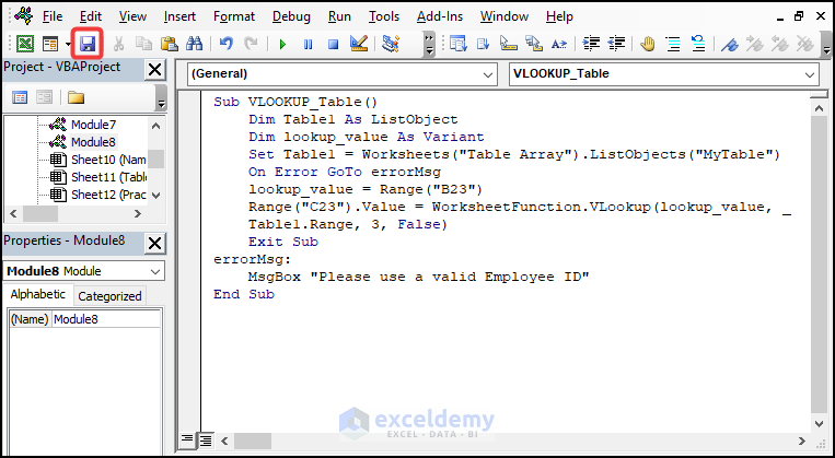
Sub VLOOKUP_Table()
Dim Table1 As ListObject
Set Table1 = Worksheets("Table Array").ListObjects("MyTable")
On Error GoTo errorMsg
lookup_value = Range("B23")
Range("C23").Value = WorksheetFunction.VLookup(lookup_value, _
Table1.Range, 3, False)
Exit Sub
errorMsg:
MsgBox "Please use a valid Employee ID"
End Sub
Code Breakdown
List of Variables Used
| Variable Name | Data Type |
|---|---|
| Table1 | ListObject |
| lookup_value | Variant |
Dim Table1 As ListObject
Set Table1 = Worksheets("Table Array").ListObjects("MyTable")- The variables are declared.
- The Set statement defines the table in the worksheet “Table Array”. Here, “MyTable”.
Range("C23").Value = WorksheetFunction.VLookup(lookup_value, _
Table1.Range, 3, False)
Exit Sub- The value of B23 is assigned to the lookup_value variable. The WorksheetFunction.VLookup method extracts data from the specified table and assigns the result to C23.
- The code exits the sub-procedure.
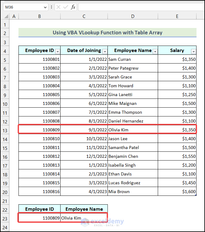
- Press ALT + F8 to open the Macro dialog box and click Run.
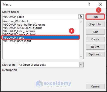
The Employee Name matching the Employee ID in B23 is displayed in C23.
Things To Remember
- By default, the InputBox function returns values as Strings.
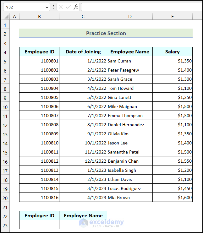
Practice Section
Practice here.
Download Practice Workbook
Download the practice workbook.
Further Readings
- Use Excel VBA VLOOKUP to Find Values in Another Worksheet
- Excel VBA to Vlookup in Another Workbook Without Opening
- Excel VBA: Working with If, IsError, and VLookup Together

