Method 1 – Create a Hyperlink Based on Cell Value in the Context Menu in Excel
In the following table, you have a list of successive month names starting from January 2021. You want to create hyperlinks to click a month name an be redirected to the sales report of that month in another sheet (Sheet2 for January-21).

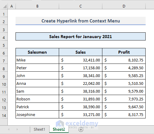
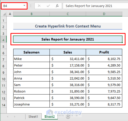
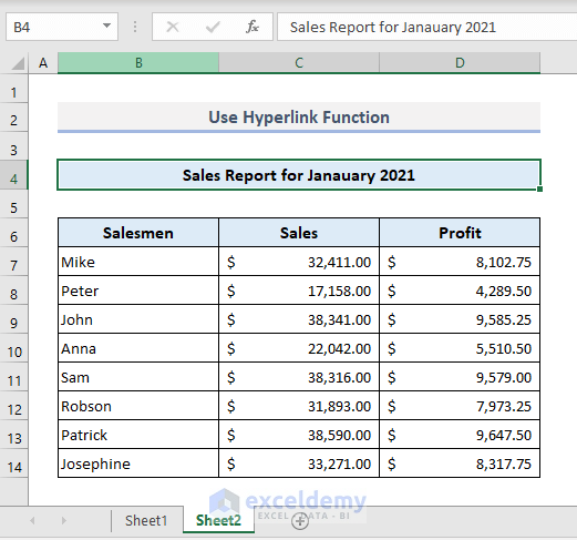
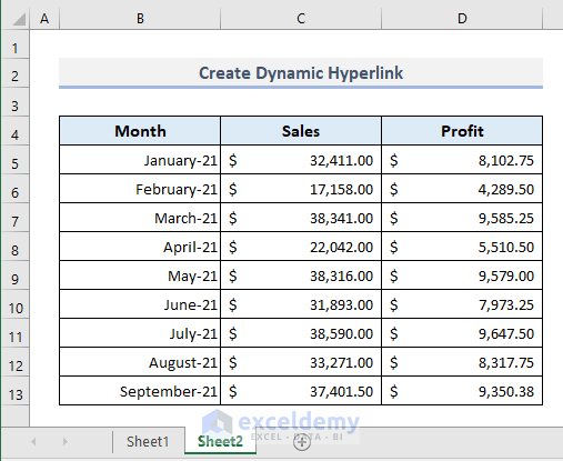
Here is Sheet2 with the sales report for January-21.
Step 1:
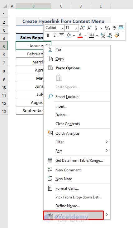
- In Sheet1, select B5.
- Right-click to open the Context Menu.
- Select Link.
A dialog box will open.
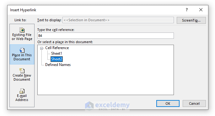
Step 2:
- In Link to, click Place in This Document.
- In ‘Type the cell reference’, enter B4.
- Select Sheet2 in Cell Reference.
- Click OK.
The hyperlink will be added to B5 in Sheet1.
Step 3:
- Click the text in B5.
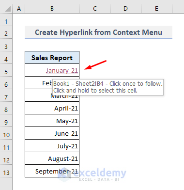
You’ll be redirected to B4 in Sheet2. Follow the same procedure to create hyperlinks for all months in Sheet1.
Read more: How to Hyperlink to Cell in Excel
Method 2 – Use the HYPERLINK function to Add a Hyperlink to Another Sheet in Excel
The generic formula of the HYPERLINK function is:
=HYPERLINK(link_location, [friendly_name])
The first argument selects the location the hyperlink will redirect you to. The Hash symbol (#) before the location keeps the search in the same workbook. The entire first argument in enclosed with Double-quotes (“ “).
The text value in the second argument is present in the cell containing the hyperlink.
Sheet1 has an additional column with the Hyperlinks header. 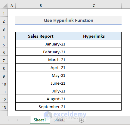
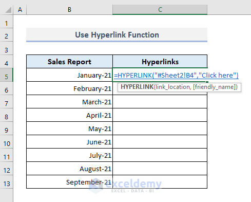
The HYPERLINK formula is:
=HYPERLINK("#Sheet2!B4","Click here")B4 in Sheet2 is referred to. The customized message is ‘Click here’.
Press Enter to see the text with the hyperlink.
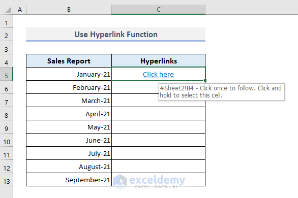
Click the hyperlinked text in C5 in Sheet1 and you’ll be redirected to B4 in Sheet2.
Read More: How to Add Hyperlink to Another Sheet in Excel
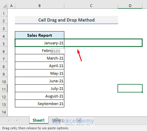
Method 3 – Applying the Cell Drag-and-Drop Method to Create a Hyperlink to Another Sheet
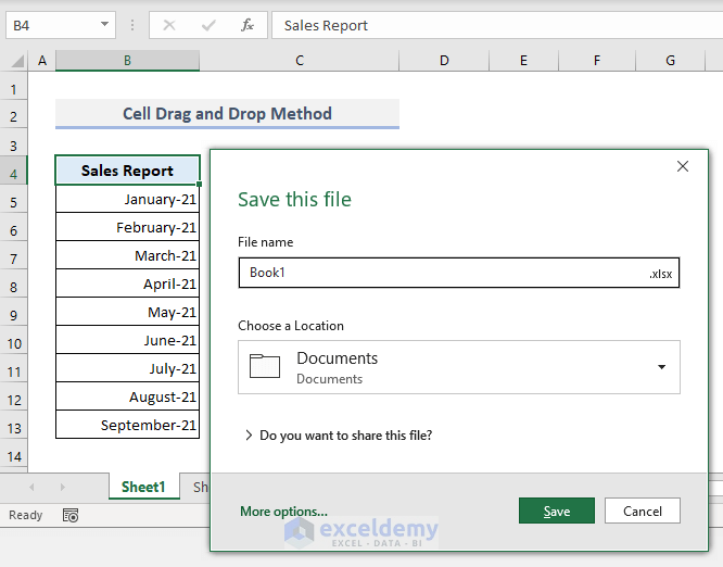
Save your workbook first.
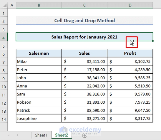
Step 1:
- Drag your mouse pointer to the cell border of the reference value.
A Plus (+) sign will be displayed.
Step 2:
- Right-click.
- Hold the button and drag it in the Sheet name in which you want to add the hyperlink.
- Press and hold ALT.
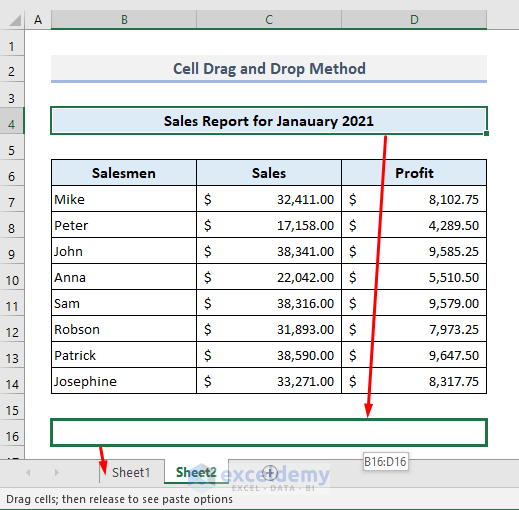
Step 3:
- In the new worksheet, release ALT.
- Drag your mouse pointer to the cell in which you’ll add the hyperlink.
- Release the mouse pointer there and the Context Menu will open.
Step 4:
- Choose ‘Create Hyperlink Here’.
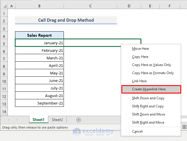
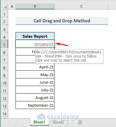
You’ll see the hyperlink.
Read More: How to Create a Drop Down List Hyperlink to Another Sheet in Excel
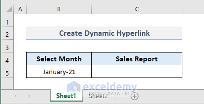
Method 4 – Create a Dynamic Hyperlink Based on the Cell Value with a Combined Formula
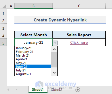
You’ll create hyperlinks based on the values of a drop-down list.
In Sheet1, B5 contains a drop-down list. In C5, embed a combined formula, using the HYPERLINK, CELL, INDEX, and MATCH functions.
After creating the hyperlinks, choose a month from the drop-down list and click the hyperlinked text in C5 to be redirected to the reference cell in (Sheet2).
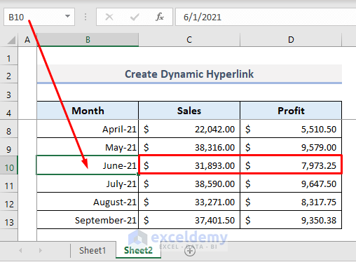
The image below is (Sheet2).
Enter formula in C5:
=HYPERLINK("#"&CELL("address",INDEX(Sheet2!B5:B13,MATCH(B5,Sheet2!B5:B13,0))),"Click here")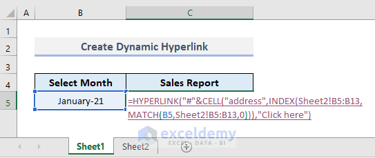
Press Enter.
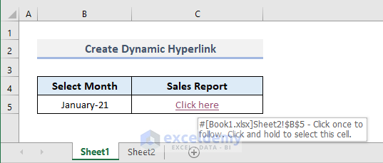
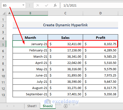
Click the hyperlink in C5 and you’ll be redirected to B5 in Sheet2.
You can select any other month (here, June-21) from the drop-down list in Sheet1.
And click the hyperlink in C5.
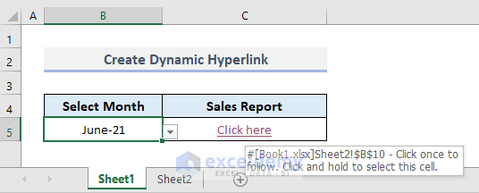
You’ll be now redirected to B10 in Sheet2.
Read More: How to Create Dynamic Hyperlink in Excel
Download Practice Workbook
Download the Excel workbook here.
You May Also Like to Explore
- How to Hyperlink to Cell in Same Sheet in Excel
- Excel Hyperlink to Cell in Another Sheet with VLOOKUP
- How to Combine Text and Hyperlink in Excel Cell
- How to Edit Hyperlink in Excel
- How to Copy Hyperlink in Excel
- How to Convert Text to Hyperlink in Excel
- How to Create Button to Link to Another Sheet in Excel
<< Go Back To Excel Hyperlink to Another Sheet | Hyperlink in Excel | Linking in Excel | Learn Excel
Get FREE Advanced Excel Exercises with Solutions!
