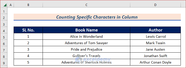
The sample dataset showcases authors and book titles:
Method 1 – Using the SUMPRODUCT Function to Count Specific Characters in a Column
1.1 Combining the SUMPRODUCT, LEN, and SUBSTITUTE Functions
To count the number of occurrences of v in C5:C9:
Steps:
- Select D11.
- Use the following formula.
- Press ENTER.
=SUMPRODUCT(LEN(C5:C9)-LEN(SUBSTITUTE(C5:C9, "v","")))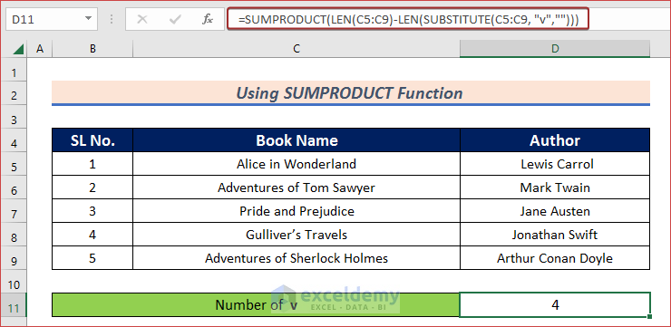
Formula Breakdown SUBSTITUTE(C5:C9, “v”,””) —> clears v in C5:C9. LEN(C5:C9)-LEN(SUBSTITUTE(C5:C9, “v”,””)) SUMPRODUCT(LEN(C5:C9)-LEN(SUBSTITUTE(C5:C9, “v”,””)))
Output: {“Alice in Wonderland”;”Adentures of Tom Sawyer”;”Pride and Prejudice”;”Gullier’s Traels”;”Adentures of Sherlock Holmes”}
{19;24;19;18;29}-{19;23;19;16;28} —> subtracts the length of C5:C9 from the updated length after replacing v.
Output: {0;1;0;2;1}
SUMPRODUCT({0;1;0;2;1}) —> sums the values and returns the result.
Output: 4
1.2 Merging the SUMPRODUCT and the EXACT Functions
Steps:
- Select D11.
- Use the following formula.
=SUMPRODUCT(--EXACT("Pride and Prejudice",C5:C9))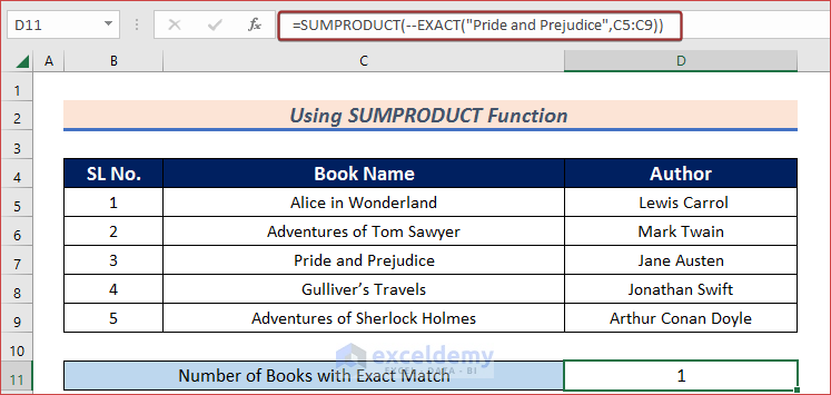
Formula Breakdown –EXACT(“Pride and Prejudice”,C5:C9) —> finds the exact match in C5:C9. SUMPRODUCT(–EXACT(“Pride and Prejudice”,C5:C9))
Output: {0;0;1;0;0}
SUMPRODUCT({0;0;1;0;0}) —> sums the values and returns the result.
Output: 1
1.3 Combining the SUMPRODUCT, ISNUMBER, and FIND Functions
To count the number of occurrences of T in C5:C9:
Steps:
- Select D11.
- Use the following formula.
=SUMPRODUCT(--ISNUMBER(FIND("T",C5:C9)))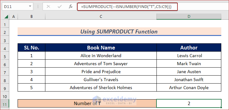
Formula Breakdown FIND(“T”,C5:C9) —> finds T in C5:C9. –ISNUMBER(FIND(“T”,C5:C9)) SUMPRODUCT(–ISNUMBER(FIND(“T”,C5:C9)))
Output: {#VALUE!;15;#VALUE!;12;#VALUE!}
–ISNUMBER({#VALUE!;15;#VALUE!;12;#VALUE!}) —> returns the number of matched values.
Output: {0;1;0;1;0}
SUMPRODUCT({0;1;0;1;0}) —> sums the values and returns the result.
Output: 2
Read More: How to Count Specific Characters in a Cell in Excel
Method 2 – Applying the COUNTIF Function to Count Specific Characters in a Column
To count the number of books starting with V in C5:C9.
Steps:
- Select D11.
- Use the following formula.
- Press ENTER.
=COUNTIF(C5:C9,"V*")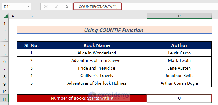
- To find book titles containing V, use the following formula:
=COUNTIF(C5:C9,"*V*")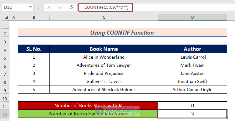
Read More: How to Count Characters in Cell Including Spaces in Excel
Method 3 – Combining the LEN and the SUBSTITUTE Functions to Count Specific Characters in a Column
Steps:
- Select D11.
- Use the following formula.
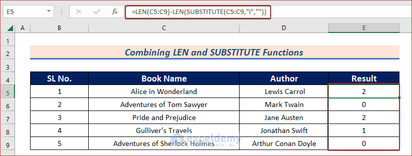
=LEN(C5:C9)-LEN(SUBSTITUTE(C5:C9,"i",""))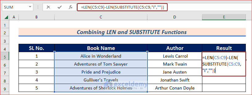
Formula Breakdown SUBSTITUTE(C5:C9,”i”,””) —> clears i in C5:C9. LEN(C5:C9)-LEN(SUBSTITUTE(C5:C9, “v”,””))
Output: {“Alce n Wonderland”;”Adventures of Tom Sawyer”;”Prde and Prejudce”;”Gullver’s Travels”;”Adventures of Sherlock Holmes”}
{19;24;19;18;29}-{17;24;17;17;29} —> subtracts the length of C5:C9 with the updated length after replacing i.
Output: {2;0;2;1;0}
- Press the ENTER to see the result.
Read More: How to Count Characters in Cell without Spaces in Excel
Method 4 – Merging the SUM and the LEFT Functions to Count Specific Characters in a Column
To count the number of books starting with A in C5:C9:
Steps:
- Select D11.
- Use the following formula.
- Press ENTER.
=SUM((LEFT(C5:C9,1)="A")*1)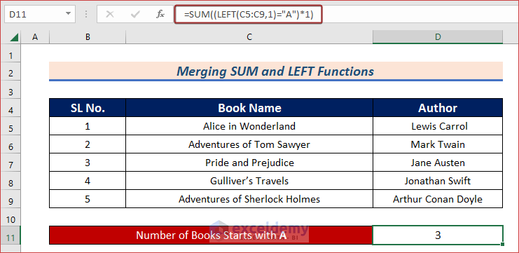
Formula Breakdown (LEFT(C5:C9,1)=”A”)*1 —> returns books starting with A in C5:C9. SUM((LEFT(C5:C9,1)=”A”)*1)
Output: {1;1;0;0;1}
SUM({1;1;0;0;1})—> sums the values and returns the result.
Output: 3
Download Practice Workbook
Download the practice workbook.
Related Articles
- How to Count Alphabet in Excel Sheet
- Excel VBA: Count Characters in Cell
- How to Count Space Before Text in Excel
- How to Count Occurrences of Character in String in Excel
<< Go Back to Count Characters in Cell | String Manipulation | Learn Excel
Get FREE Advanced Excel Exercises with Solutions!

Amazing! Thanks so much for this formula! The 1a did the trick. Thanks again 🙂