Excel CEILING.MATH Function: Syntax and Arguments
Summary:
- The CEILING.MATH function rounds a specified number up to the nearest integer or nearest specified multiple of significance.
- This function rounds all positive numbers with decimal places up to the nearest integer as its default feature.
- This function rounds all negative numbers with decimal places up towards zero to the nearest integer as its default feature.
- Available from Excel 2013.
Syntax:
The syntax or formula for the CEILING.MATH function of Excel is
=CEILING.MATH(number, [significance], [mode])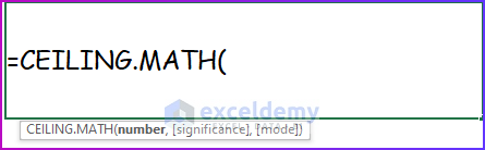
Arguments:
| Argument | Required or Optional | Value |
|---|---|---|
| Number | Required | The ‘number’ is the number of interests that you would like to round up. |
| Significance | Required | The ‘significance’ is optional and specifies the multiple to which the number of interests will round up. |
| Mode | Optional | The ‘mode’ is an optional argument and controls the way Excel handles the negative numbers. |
Return:
This function will return the nearest rounded integer of a specific number.
Excel FLOOR.MATH Function: Syntax and Arguments
Summary:
- The FLOOR.MATH function also rounds a specified number down to the nearest integer or nearest specified multiple of significance.
- The function also provides additional options for rounding negative numbers.
- The FLOOR.MATH function allows one to reverse the direction of the rounding for negative numbers by specifying the mode.
- Available from Excel 2013.
Syntax:
The syntax or formula for the FLOOR.MATH function of Excel is
=FLOOR.MATH(number, [significance], [mode])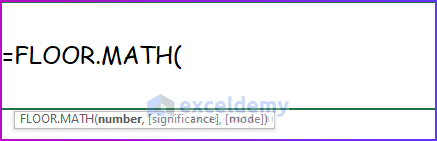
Arguments:
| Argument | Required or Optional | Value |
|---|---|---|
| Number | Required | The ‘number’ is the number of interests that you would like to round down. |
| Significance | Required | The ‘significance’ is optional and specifies the multiple to which the number of interests will round down. |
| Mode | Optional | The ‘mode’ is an optional argument and controls the way Excel handles the negative numbers. |
Return:
This function will return the nearest rounded integer of a specific number.
How to Use CEILING.MATH and FLOOR.MATH Functions in Excel
We can use these functions in order to allow specific control over the way to round the negative numbers. By specifying the mode, one can control if negative numbers will round towards 0 or away from 0. This depends on what one’s rounding needs are.
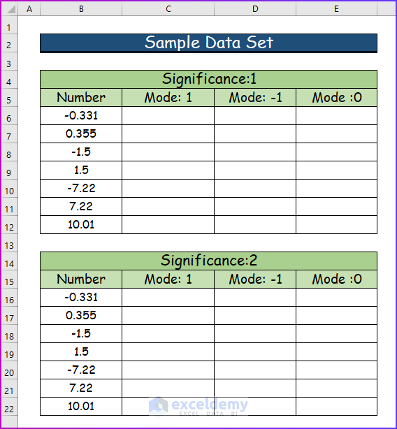
We will use the following sample dataset for illustration.
Example 1 – Using CEILING.MATH Function
We will use the CEILING.MATH function to round up using first a significance of 1 and a mode of 1. Then, a significance of 1 and a mode of -1 and a significance of 1 and a mode of 0. We are then going to use the CEILING.MATH function in conjunction with a significance of 2 and a mode of 1. Then, a significance of 2 and a mode of -1 and a significance of 2 and a mode of 0. The detailed steps are as follows.
Step 1:
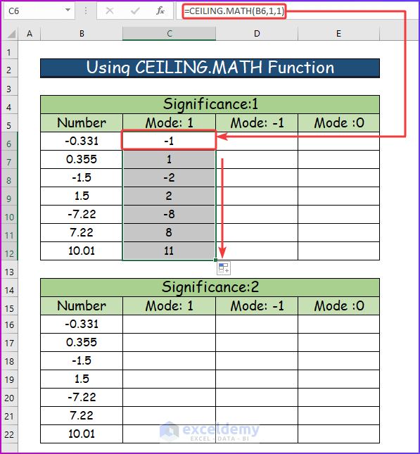
We want to see the effect of a significance of 1 and a mode of 1.
- In cell C6, enter the following formula:
=CEILING.MATH(B6,1,1)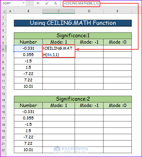
Step 2:
- Press Ctrl + Enter,
The formula will deliver a value of -1, which rounds the negative number -0.331 away from 0.
- Use AutoFill to drag the formula down.
Since we have used relative references. We will get the following results.
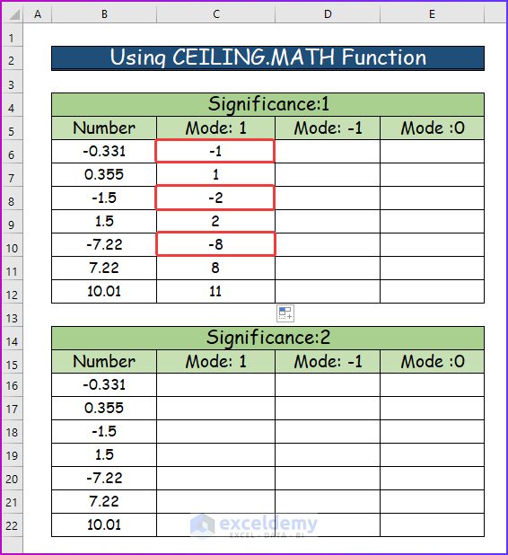
Step 3:
- Since we specified the significance of 1, which is also the default significance, the formula will round the positive numbers towards the nearest integer. That, in the case of 355 is 1, 5 is 2, 7.22 is 8, and 10.01 is 11.
- Since we specified a mode of 1, the formula will round the negative numbers away from 0. So, the formula will round away -0.331 from 0 to -1, -1.5 to -2 and -7.22 to -8. You can see it in the following image.
Step 4:
In cell D6, we want to see what will happen if we specify a significance of 1, and a mode of -1. So,
- In cell D6, enter the following formula:
=CEILING.MATH(B6,1,-1)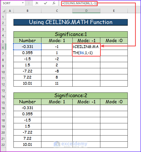
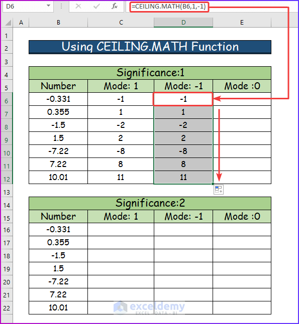
Step 5:
- Press Ctrl + Enter.
The formula will deliver a value of -1 again, which rounds the negative number -0.331 away from 0.
- Drag the formula down.
Since we used relative references and we will get the following results.
We can see that specifying either a positive number or a negative number for the mode results in negative numbers and will round the number away from 0.
Step 6:
In cell E6, we want to see what will happen if we specify a significance of 1, and a mode of 0.
- In cell E6, enter the following formula:
=CEILING.MATH(B6,1,0)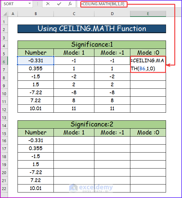
Step 7:
- Press Ctrl + Enter.
A value of 0, which rounds the negative number toward 0.
- Drag down the Fill Handle to see the results for the lower cells of the column.
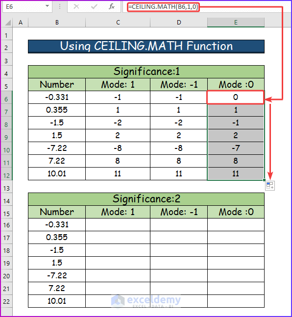
We can see in comparison to a mode of -1 and 1, a mode of 0 rounds the negative numbers towards 0. So, –0.331 is rounded towards 0 and thus 0 is delivered, -1.5 is rounded towards 0 and thus -1 is delivered. -7.22 is also rounded towards 0 and thus -7 is delivered when using 0 as the mode.
Step 8:
To find out what will happen if we use a significance of 2 and a mode of 1,
- In cell C16, enter the following formula:
=CEILING.MATH(B16,2,1)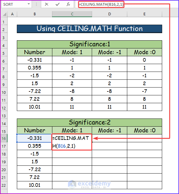
Step 9:
- Press Ctrl + Enter.
The formula will deliver a value of -2, which rounds the negative number away from 0. Since the mode specified was 1 and the formula delivers -2 since this is the multiple of 2 considerations, as specified by the significance.
- Use AutoFill to drag the formula down.
Since we have used relative references, we will get the following results.
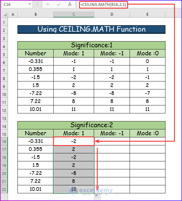
Step 10:
- Since we specified the significance of 2, the positive numbers are rounded up towards the nearest multiple of 2, which in the case of355 is 2, 1.5 is 2, 7.22 is 8, and 10.01 is 12.
- Also, since we specified a mode of 1, the negative numbers are rounded away from 0 with a multiple of 2 in consideration due to the significance, so -0.331 is rounded away from 0 to -2, –5 to -2, -7.22 to -8.
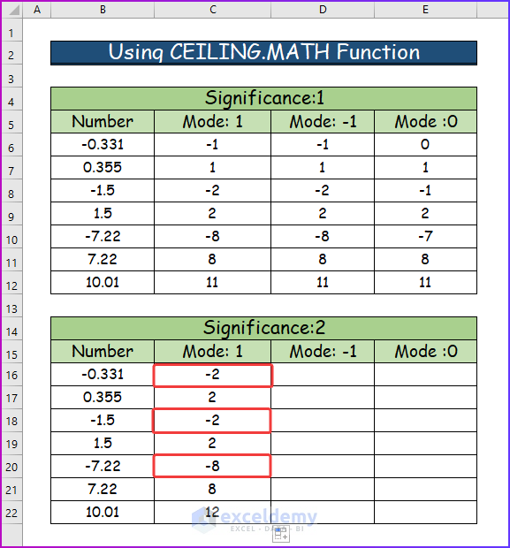
Step 11:
We want to see what will happen if we specify a significance of 2 and a mode of -1.
- In cell D16, enter the following formula:
=CEILING.MATH(B16,2,-1)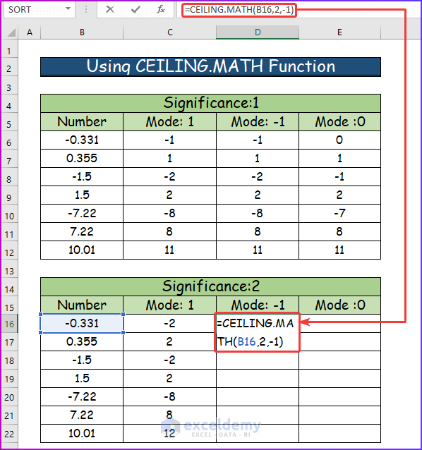
Step 12:
- Press Ctrl + Enter.
A value of -2, is delivered again, which rounds the negative number -0.331 away from 0 since the mode specified was -1 and -2 is delivered since this is the multiple of 2 considerations as specified by the significance.
- Use the Fill Handle to show the result of the other cells in that column.
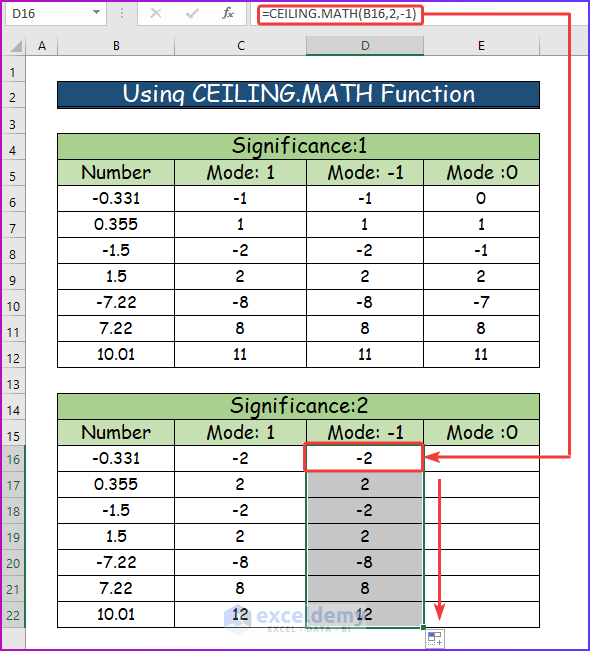
Step 13:
We can thus see that specifying either a positive number or a negative number for the mode results in negative numbers being rounded away from 0 and in this case, since significance was 2, the multiple of 2 is considered when rounding.
We want to see what will happen if we specify a significance of 2 and a mode of 0.
- In cell E16, enter the following formula:
=CEILING.MATH(B16,2,0)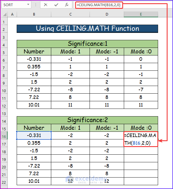
Step 14:
- Press Ctrl + Enter.
The formula will deliver a value of 0, which rounds the negative number toward 0.
- Drag down the formula to get the following results.
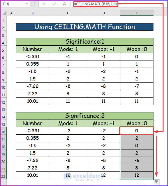
We can now see in comparison to a mode of -1 and 1, a mode of 0 rounds the negative numbers towards 0 with the multiple of 2 set by the significance taken into consideration, so –0.331 is rounded towards 0 and thus 0 is delivered, -1.5 is rounded towards 0 and thus 0 is delivered and -7.22 is also rounded towards 0 and thus -6 is delivered when using 0 as the mode and 2 as the significance.
Example 2 – Using FLOOR.MATH Function
In this example, we will use the FLOOR.MATH function to round down using first a significance of 1 and a mode of 1, then a significance of 1 and a mode of -1, and a significance of 1 and a mode of 0. We are then going to use the FLOOR.MATH function in conjunction with a significance of 2 and a mode of 1, a significance of 2 and a mode of -1, and a significance of 2 and a mode of 0. Go through the following steps for the detailed procedure.
Step 1:
- We want to see the effect of a significance of 1 and a mode of 1. So, in cell C6, enter the following formula:
=FLOOR.MATH(B6,1,1)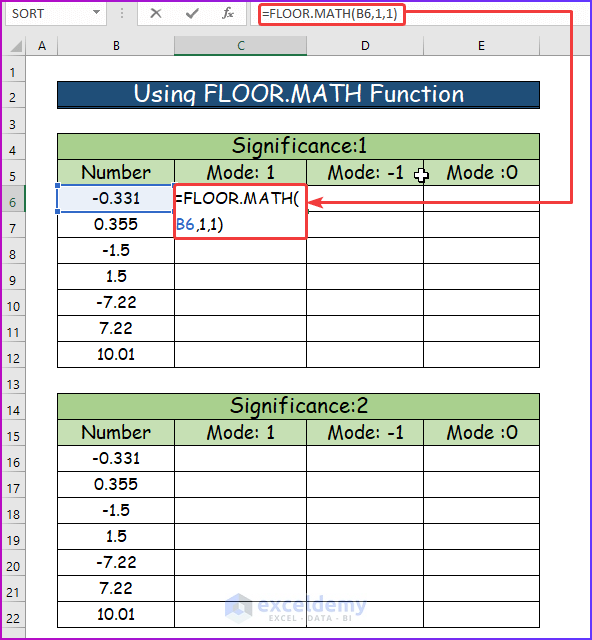
Step 2:
- Press Ctrl + Enter.
A value of 0, is delivered, which rounds the negative number -0.331 toward 0.
- Drag the formula down using AutoFill.
Since we have used relative references, you will get the following results.

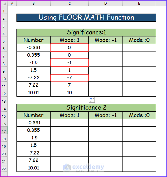
Step 3:
- Since we specified the significance of 1, which is also the default significance, the positive numbers are rounded down towards the nearest integer, which in the case of 355 is 0, 1.5 is 1, 7.22 is 7, and 10.01 is 10.
- Also, since we specified a mode of 1, the negative numbers are rounded toward 0, so -0.331 is rounded toward 0 to 0, -1.5 to -1, and -7.22 to -7. This is emphasized below, and we can compare the difference to the CEILING.MATH treatment of the negative numbers at the significance of 1 and mode of 1.
Step 4:
We want to see what will happen if we specify a significance of 1, and a mode of -1.
- In cell D6, enter the following formula:
=FLOOR.MATH(B6,1,-1)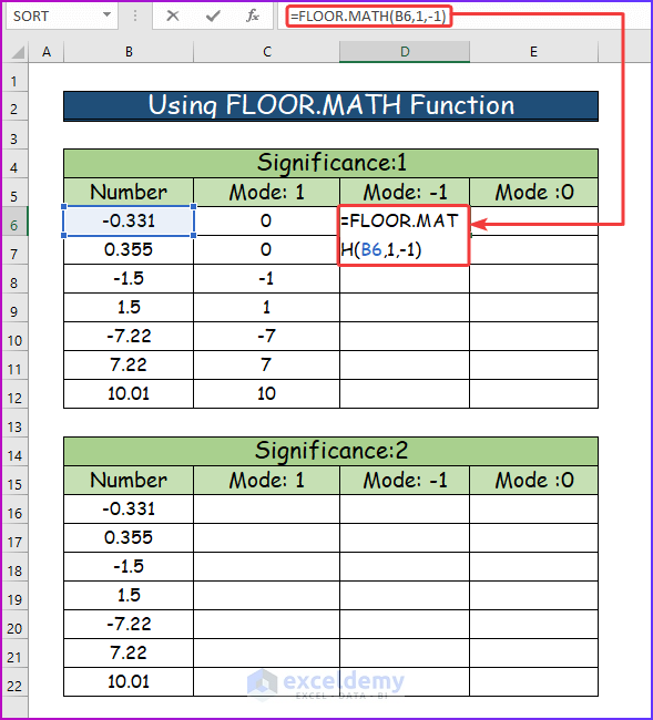
Step 5:
- Press Ctrl + Enter.
The formula will deliver a value of 0, which rounds the negative number -0.331 towards 0.
- Drag the formula down to get the following results.
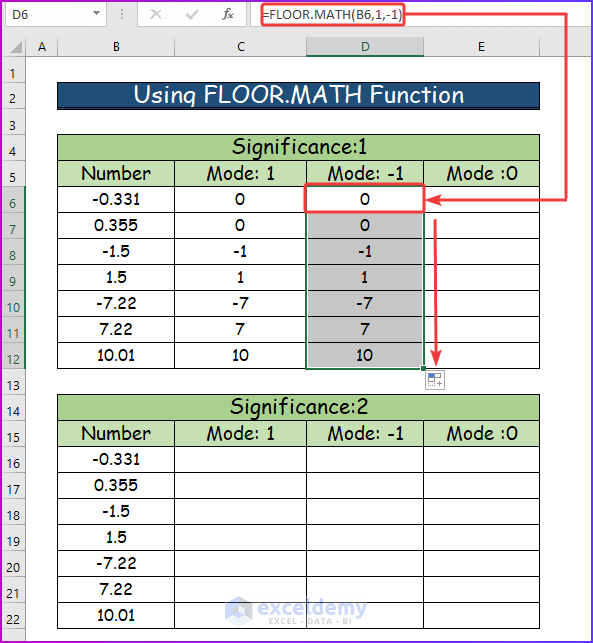
Step 6:
- Specifying either a positive number or a negative number for the mode results in negative numbers being rounded towards 0.
- We want to see what will happen if we specify a significance of 1, and a mode of 0. In cell E6, enter the following formula:
=FLOOR.MATH(B6,1,0)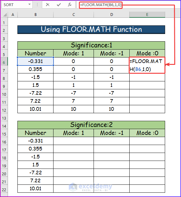
Step 7:
- Press CTRL+ ENTER.
The formula will deliver a value of -1, which rounds the negative number away from 0.
- Drag the formula down to the following results.
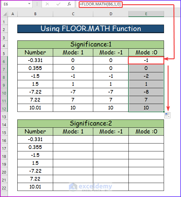
In comparison to a mode of -1, and 1, a mode of 0 rounds the negative numbers away from 0, so –0.331 is rounded away. Similarly, -1 is delivered, -1.5 is rounded away from 0, and thus -2 is delivered, and -7.22 is also rounded away from 0, and thus -8 is delivered when using 0 as the mode. We can also compare the difference in the way the CEILING.MATH function handles the negative numbers with the respective modes.
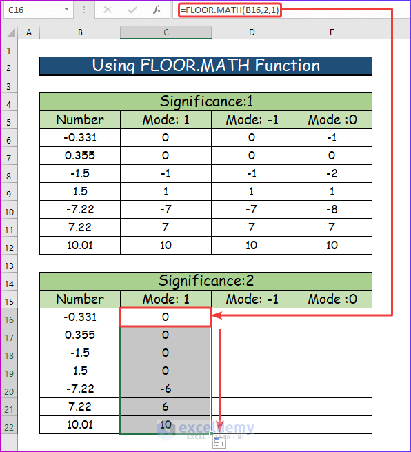
Step 8:
We will see what will happen if we use a significance of 2 and a mode of 1.
- In cell B16, enter the following formula:
=FLOOR.MATH(B16,2,1)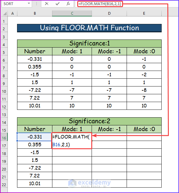
Step 9:
- Press CTRL + ENTER.
We will see a value of 0. That rounds the negative number towards 0 since the mode specified was 1, and 0 is delivered since this is the nearest multiple of 2 as specified by the significance.
- Drag down the formula and we will get the following results.
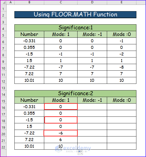
Step 10:
- Since we specified the significance of 2, the formula will round down the positive numbers towards the nearest multiple of 2, which in the case of 355 is 0, 1.5 is 0, 7.22 is 6, and 10.01 is 10.
- Also, since we specified a mode of 1, the negative numbers are rounded toward 0 with a multiple of 2 in consideration due to the significance, so -0.331 is rounded towards 0 to 0, -1.5 to 0, and -7.22 to -6. This can be seen below.
Step 11:
We will see what will happen if we specify a significance of 2 and a mode of -1.
- In cell D16, enter the following formula:
=FLOOR.MATH(B16,2,-1)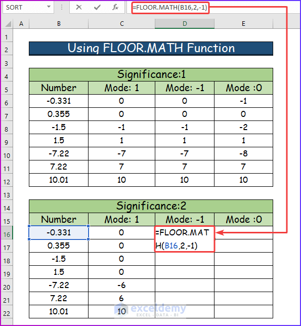
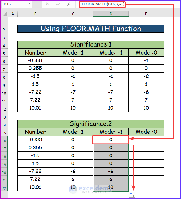
Step 12:
- Press CTRL + ENTER.
You will see a value of 0, which rounds the negative number -0.331 towards 0, to the nearest multiple of 2 as specified by the significance, which is 0 in this case.
- Use Fill Handle to drag the formula down and we will get the following results.
Specifying either a positive number or a negative number for the mode results in negative numbers being rounded towards 0, and in this case, since significance was 2, the formula will consider the multiple of 2 while rounding.
Step 13:
In cell E16, we want to see what will happen if we specify a significance of 2, and a mode of 0.
- In cell E16, we enter the following formula:
=FLOOR.MATH(B16,2,0)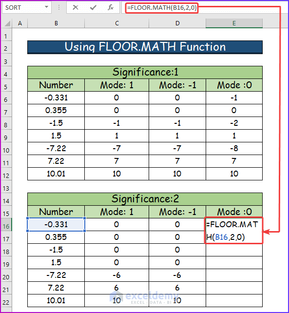
Step 14:
- Press CTRL +ENTER.
You will see a value of -2, which rounds the negative number away from 0.
- Drag the formula down to get the following results.
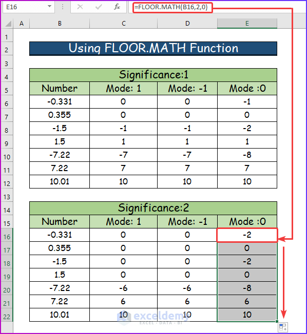
In comparison to a mode of -1, and 1, a mode of 0 rounds the negative numbers away from 0 with the multiple of 2 set by the significance taken into consideration. So, –0.331 is rounded away from 0, and thus -2 is delivered, -1.5 is rounded away from 0, and thus -2 is delivered, and -7.22 is also rounded away from 0, and thus -8 is delivered when using 0 as the mode, and 2 as the significance.
Download Practice Workbook
Related Articles
<< Go Back to Excel Functions | Learn Excel
Get FREE Advanced Excel Exercises with Solutions!
