The dataset contains Products, Customers and Quantity sold.
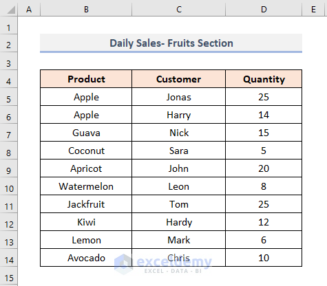
Cell values in Column B are the base values.
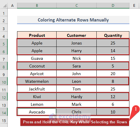
Method 1 – Alternate Row Color Manually Based on the Cell Value in Excel
Steps
- Select alternate rows by pressing CTRL.
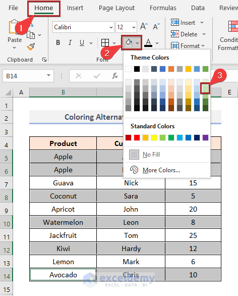
- Go to the Home tab.
- Select Fill Color in Font.
- Choose Green, Accent 6, Lighter 60%.
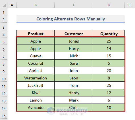
This is the output.
Method 2 – Using the Format as Table Option in Excel
Steps
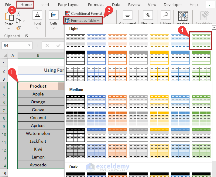
- Select the dataset. Here, B4:D14.
- Go to the Home tab.
- Select Format as Table in Styles.
- Choose Light Green, Table Style Light 7.
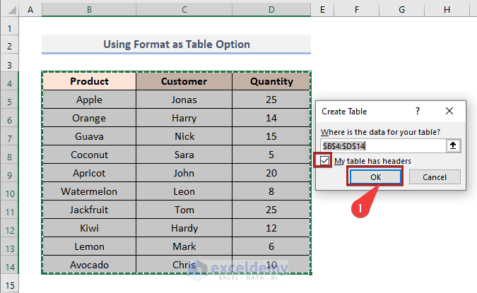
- In the Create Table dialog box, check My table has headers.
- Click OK.
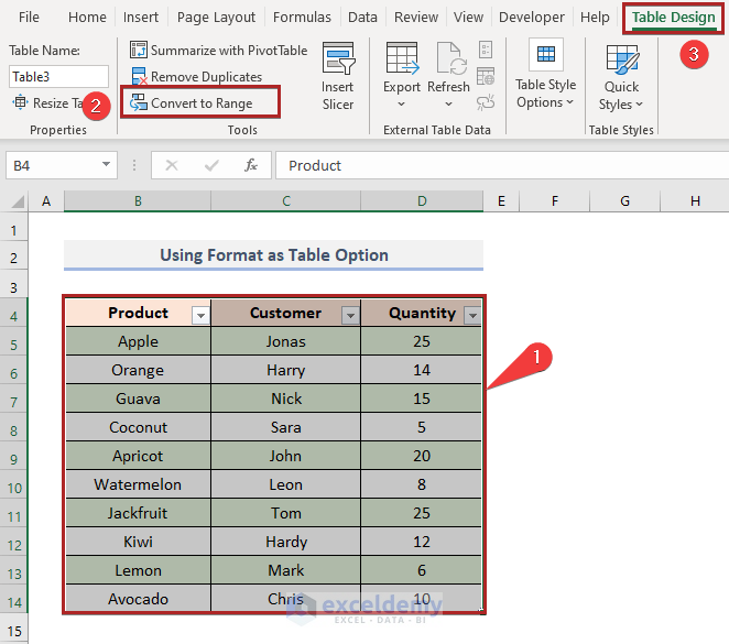
- Select the whole table. Here, B4:D14.
- Go to Table Design.
- Select Convert to Range in Tools.
- Click Yes in the warning box.
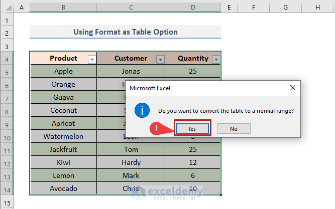
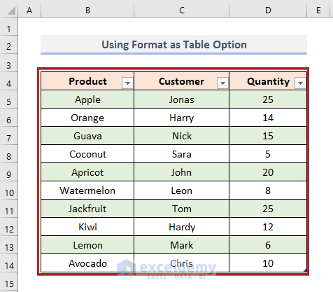
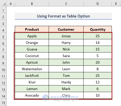
This is the output.
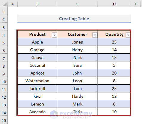
Method 3 – Creating a Table to Alternate Row Color Based on the Cell Value in Excel
Steps
- Select B4:D14.
- Go to the Insert tab.
- Select Table in Tables.
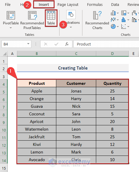
- In the Create Table dialog box, click OK.
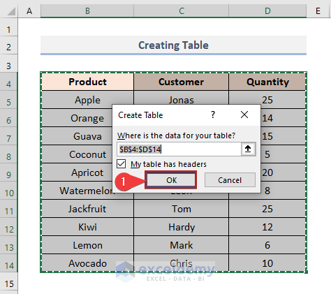
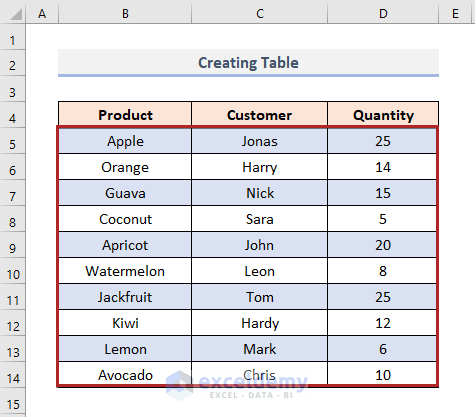
The data range is converted into the following table with alternate row colors.
- To convert the table into the range, follow the steps in Method 2.
Read More: How to Alternate Row Colors in Excel Without Table
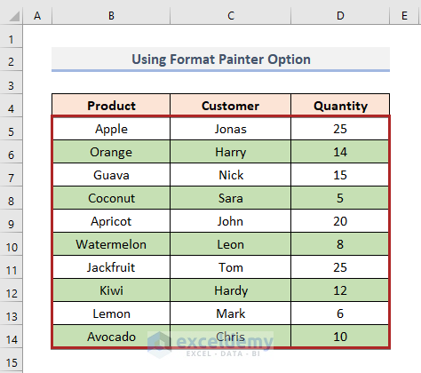
Method 4 – Using the Format Painter Option
Steps
- Select the second row in the range and go to the Home tab.
- Select Fill Color in Font.
- Choose Green, Accent 6, Lighter 60%.
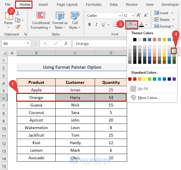
One row has no color and the other row has color. Use the Format Painter to copy this format.
- Select the first two rows: 5 and 6.
- Select Format Painter in Clipboard.
- Drag the Format Painter sign down and to the right side.
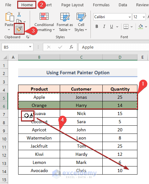
This is the output.
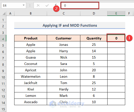
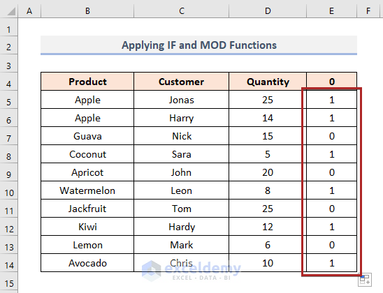
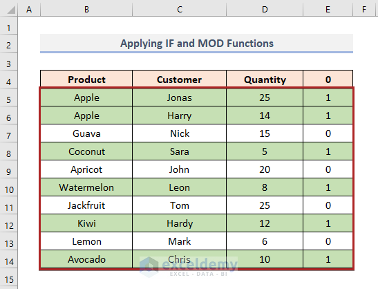
Method 5 – Applying the IF and MOD Functions
Steps
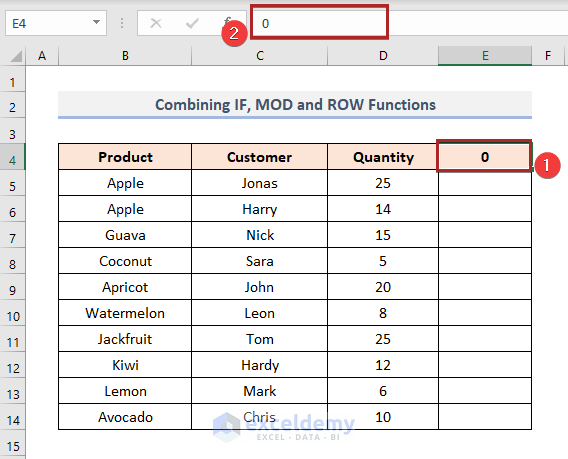
- Select E4 and enter Zero (0) into the cell.
0
- Press ENTER.
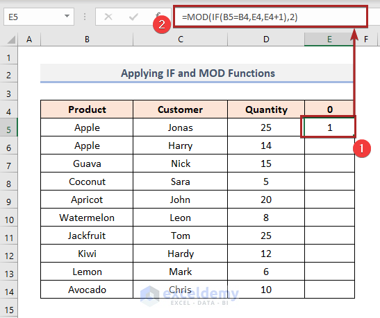
- Select E5 and enter the following formula.
=MOD(IF(B5=B4,E4,E4+1),2)
Formula Breakdown
IF(B5=B4, E4, E4+1): The IF function checks the value of B5 and B4. If both values match, the function returns the value of E4. Otherwise, it will add 1 to the value of E4.
MOD(IF(B5=B4, E4, E4+1),2): The MOD function divides the result of the IF function by 2 and shows the value of the remainder.
- Press ENTER.
- Double-click the Fill Handle icon to copy the formula to the rest of the cells.
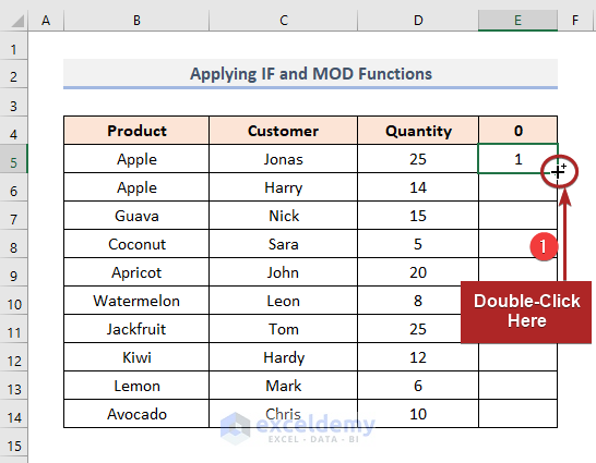
This is the output.
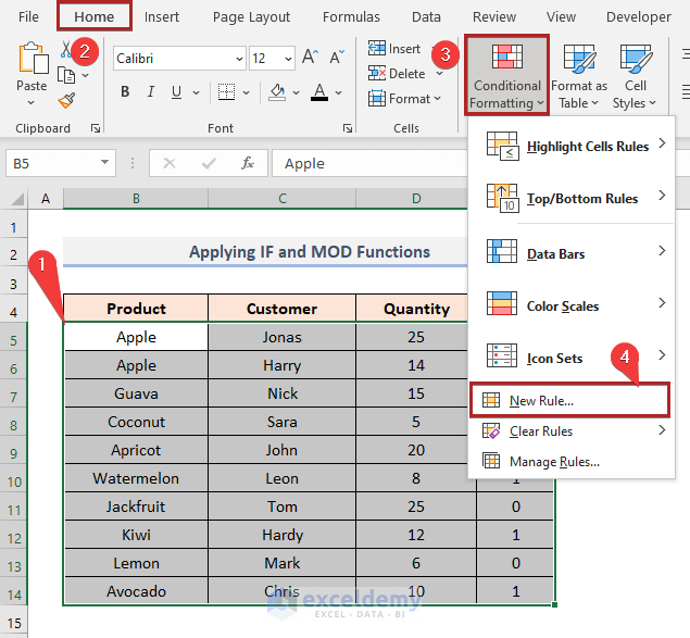
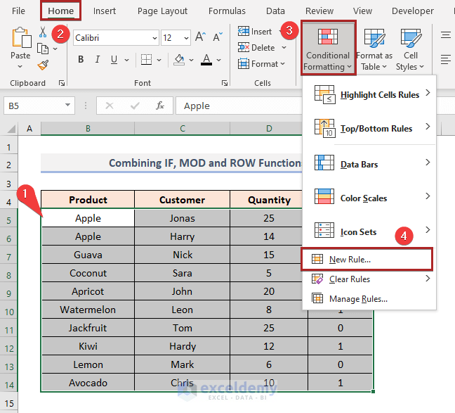
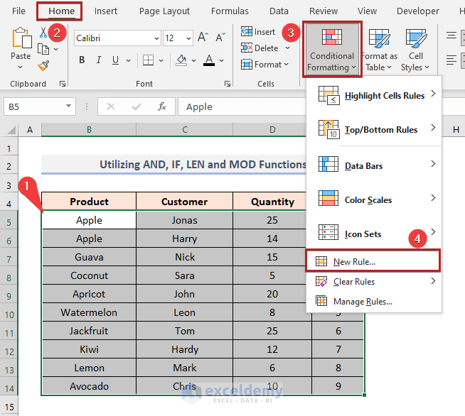
- Select B5:E14.
- Go to the Home tab
- Click the drop-down arrow of Conditional Formatting in Styles.
- Select New Rule.
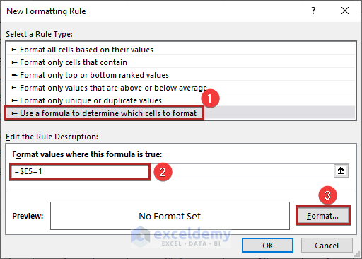
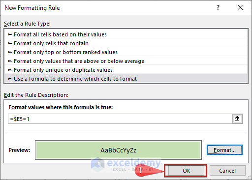
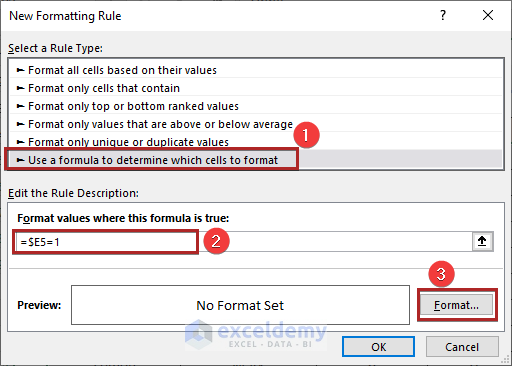
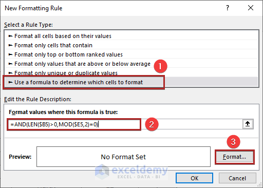
- In the New Formatting Rule dialog box, select Use a formula to determine which cells to format in Select a Rule Type.
- Enter the following formula in Format values where the formula is true.
=$E5=1
- Click Format.
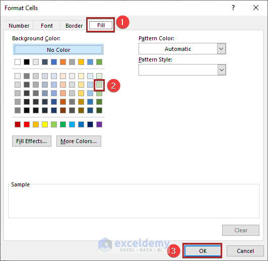
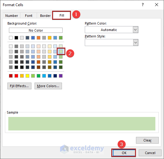
- In the Format Cells dialog box, select Fill.
- Choose a color. Here, Green, Accent 6, Lighter 60%.
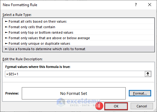
- Click OK.
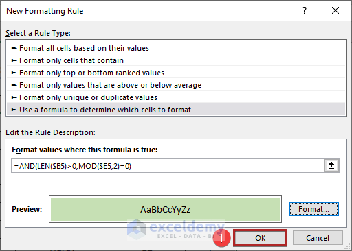
- Click OK to close the New Formatting Rule dialog box.
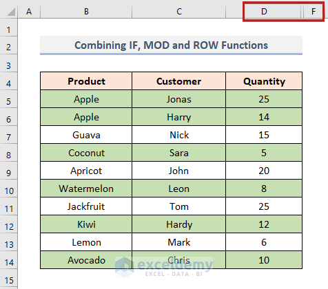
- Right-click Column E.
- Select Hide.
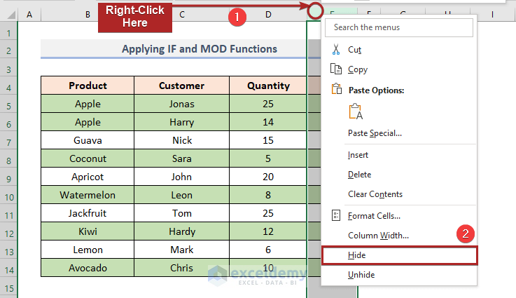
The extra column is hidden. This is the final output.

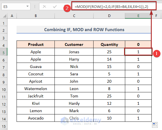
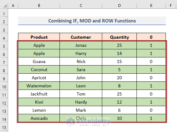
Method 6 – Combining the IF, MOD, and ROW Functions
Steps
- Select E4 and enter Zero (0).
0
- Press ENTER.
- Select E5 and enter the following formula.
=MOD(IF(ROW()=2,0,IF(B5=B4,E4,E4+1)),2)
Formula Breakdown
ROW(): The ROW function returns the row number. Here, 5.
IF(B5=B4, E4, E4+1): The IF function checks the value of B5 and B4. If both values match, the function returns the value of E4. Otherwise, it will add 1 to the value of E4.
IF(ROW()=2,0,IF(B5=B4,E4, E4+1)): The IF function checks whether the row number is equal to 2. If the logic is True, the function returns 0. If the logic is False, the function returns the result of the second IF function.
MOD(IF(ROW()=2,0,IF(B5=B4,E4, E4+1)),2): The MOD function divides the result of the IF function by 2 and shows the value of the remainder.
- Press ENTER.
- Select B5:E14.
- Go to the Home tab
- Click the drop-down arrow of Conditional Formatting in Styles.
- Select New Rules.
- In the New Formatting Rule dialog box, select Use a formula to determine which cells to format in Select a Rule Type.
- Enter the following formula in Format values where the formula is true.
=$E5=1
- Click Format.
- In Format Cells, select Fill.
- Choose a color. Here, Green, Accent 6, Lighter 60%.
- Click OK.

- Click OK to close the New Formatting Rule dialog box.
Alternate row colors based on the value are displayed.
- Follow the steps of Method 5 to hide the extra column.
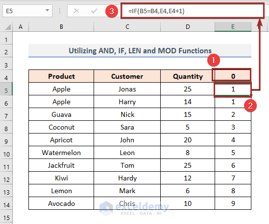
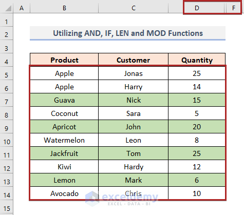
Method 7 – Utilizing the AND, IF, LEN, and MOD Functions
Steps
- Select E4 and enter Zero (0).
0
- Press ENTER.
- Select E5 and enter the following formula.
=IF(B5=B4,E4,E4+1)
Formula Breakdown
IF(B5=B4, E4, E4+1): The IF function checks the value of cell B5 and B4. If both values match, the function returns the value of E4. Otherwise, it will add 1 to the value of E4.
- Press ENTER.
- Select B5:E14.
- Go to the Home tab
- Click the drop-down arrow of Conditional Formatting in Styles.
- Select New Rules.
- In the New Formatting Rule dialog box, select Use a formula to determine which cells to format in Select a Rule Type.
- Enter the following formula in Format values where the formula is true.
=AND(LEN($B5)>0,MOD($E5,2)=0)
Formula Breakdown
LEN($B5): The LEN function counts the length of the cell value. Here, 5.
MOD($E5,2): This function divides the value of E5 by 2 and shows the value of the remainder. Here, 1.
AND(LEN($B5)>0, MOD($E5,2)=0): In this formula, the AND function checks whether the value of the LEN function is greater than 5 and the result of the MOD function is equal to 0. If the logic is True, the row will show the selected color.
- Click Format.
- In Format Cells, select Fill.
- Choose a color. Here, Green, Accent 6, Lighter 60%.
- Click OK.
- Click OK to close the New Formatting Rule dialog box.
This is the output.
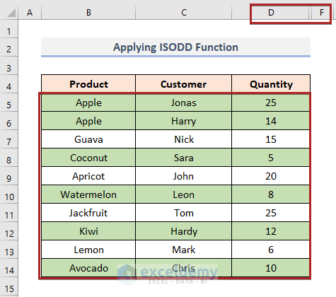
Method 8 – Applying the ISODD Function to Alternate Row Color Based on the Cell Value in Excel
Steps
- Select E4 and enter Zero (0).
0
- Press ENTER.
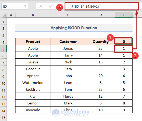
- Select E5 and enter the following formula.
=IF(B4=B5,E4,SUM(E4,1))
Formula Breakdown
SUM(E4,1): The SUM function adds 1 to the value of E4 and returns 1.
IF(B4=B5,E4,SUM(E4,1)): The IF function checks the value of B5 and B4. If both values match, the function returns the value of E4. If the logic is False, it returns the result of the SUM function.
- Press ENTER.
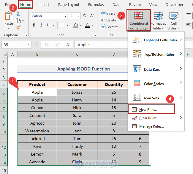
- Select B5:E14.
- Go to the Home tab
- Click the drop-down arrow of Conditional Formatting in Styles.
- Select New Rules.
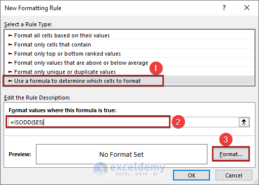
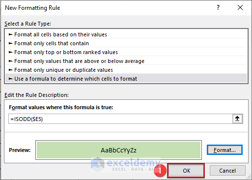
- In the New Formatting Rule dialog box, select Use a formula to determine which cells to format in Select a Rule Type.
- Enter the following formula in Format values where the formula is true.
=ISODD($E5)
ISODD will determine if the corresponding cell value is odd. If it is odd, it will return TRUE. If the logic is TRUE the row will show the selected color.
- Click Format.
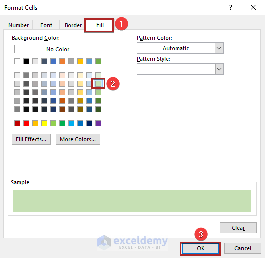
- In Format Cells, select Fill.
- Choose a color. Here, Green, Accent 6, Lighter 60%.
- Click OK.
- Click OK to close the New Formatting Rule dialog box.
This is the output.
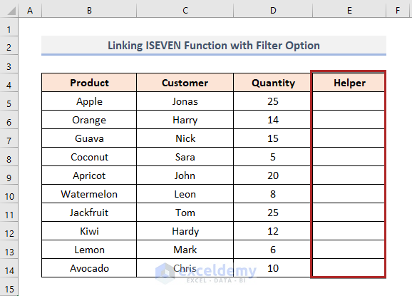
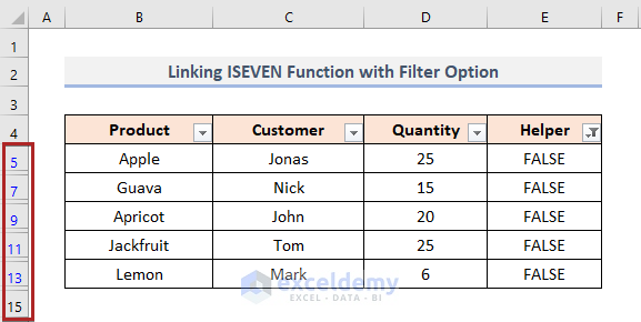
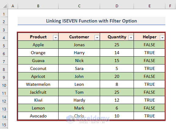
Method 9 – Combining the ISEVEN Function with the Filter Option
Steps
- Add a Helper column.
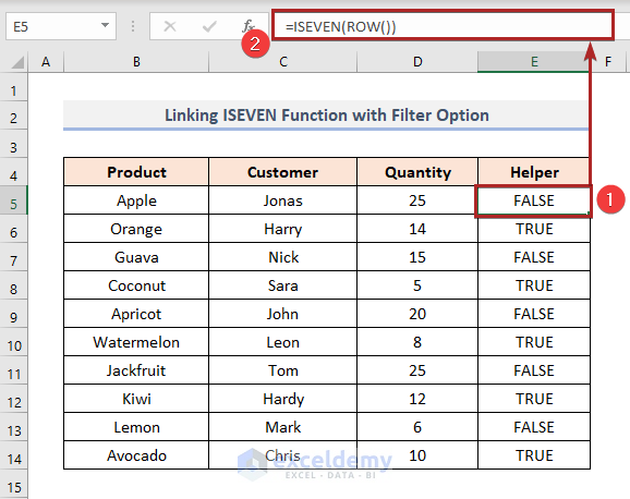
- Select E5 and enter the following formula.
=ISEVEN(ROW())
The ROW function returns the row number. ISEVEN will determine if the corresponding row number is even. If it is even, it will return TRUE. Otherwise, FALSE.
- Press ENTER.
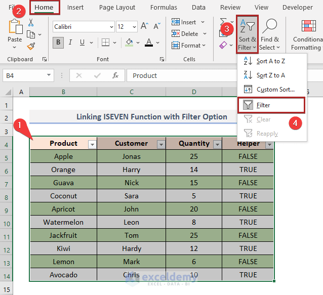
- Select the dataset: B4:E14.
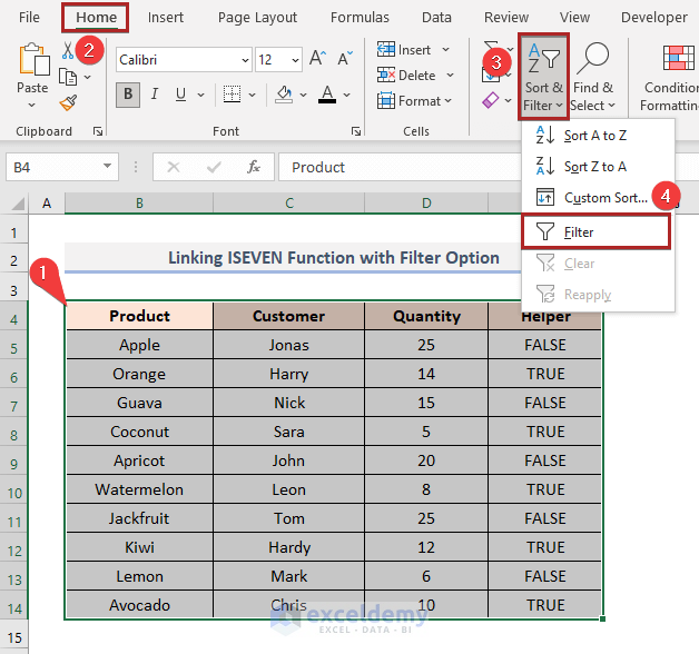
- Go to the Home tab.
- Select Sort & Filter in Editing.
- Choose Filter.
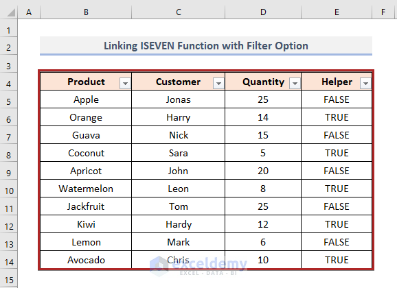
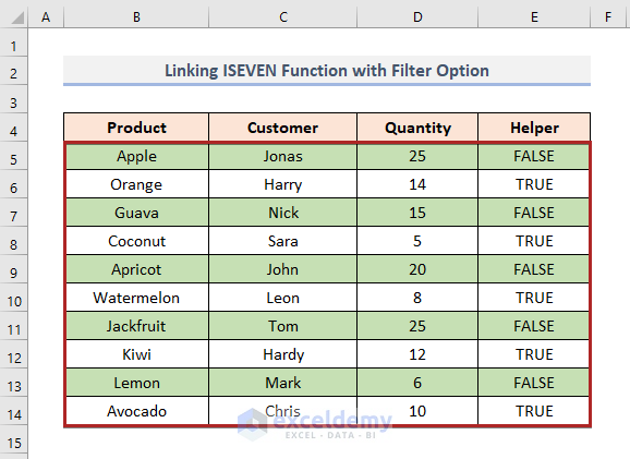
This is the filtered table.
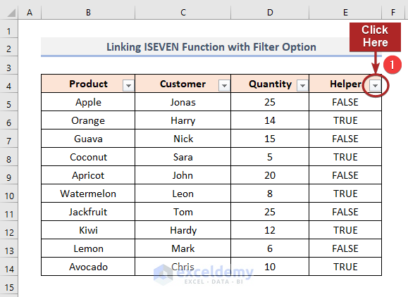
- Click the dropdown symbol in the Helper column.
- Uncheck TRUE and click OK.
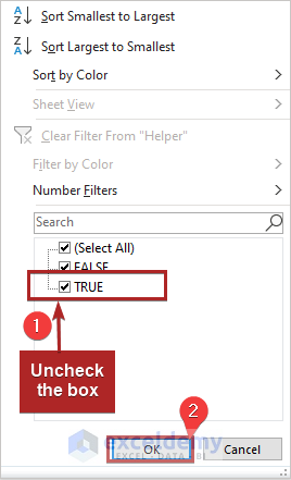
The rows with TRUE will be hidden.
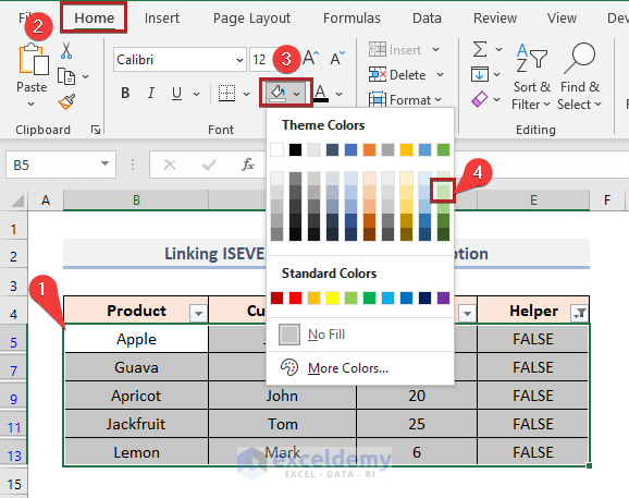
- Select the unhidden rows in the dataset.
- Go to the Home tab.
- Select Fill Color in Font.
- Choose Green, Accent 6, Lighter 60%.
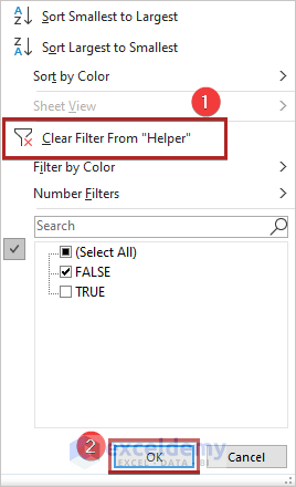
- Click the dropdown symbol in the Helper column.
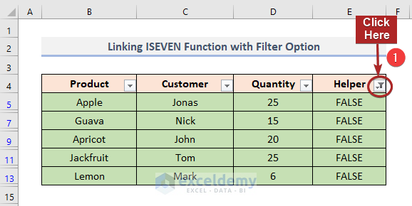
- Select Clear Filter From “Helper”.
- Click OK.
Alternate row colors are displayed.
- Select the whole dataset including the header row.
- Go to the Home tab.
- Select Sort & Filter in Editing.
- Uncheck Filter.
This is the output.
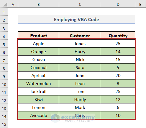
Method 10 – Using a VBA Code to Alternate Row Color Based on the Cell Value in Excel
Steps
- Press ALT+F11.
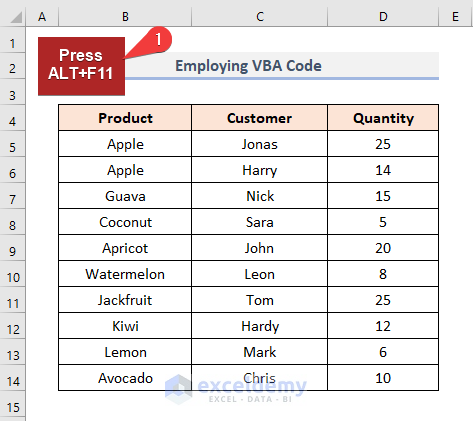
- The Microsoft Visual Basic for Applications window will open.
- Go to the Insert tab.
- Select Module.
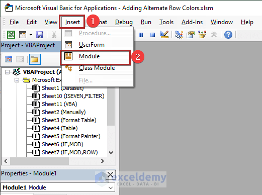
- Enter the code below.
Sub Alternate_Row_Color()
Dim y As Integer
For y = 1 To Selection.Rows.Count
If y Mod 2 = 0 Then
Selection.Rows(y).Interior.Color = RGB(198, 224, 180)
End If
Next
End Sub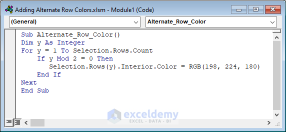
y is declared as Integer and the FOR loop will work for each row. The IF statement will ensure that if the row number is divisible by 2 or even, it will be colored.
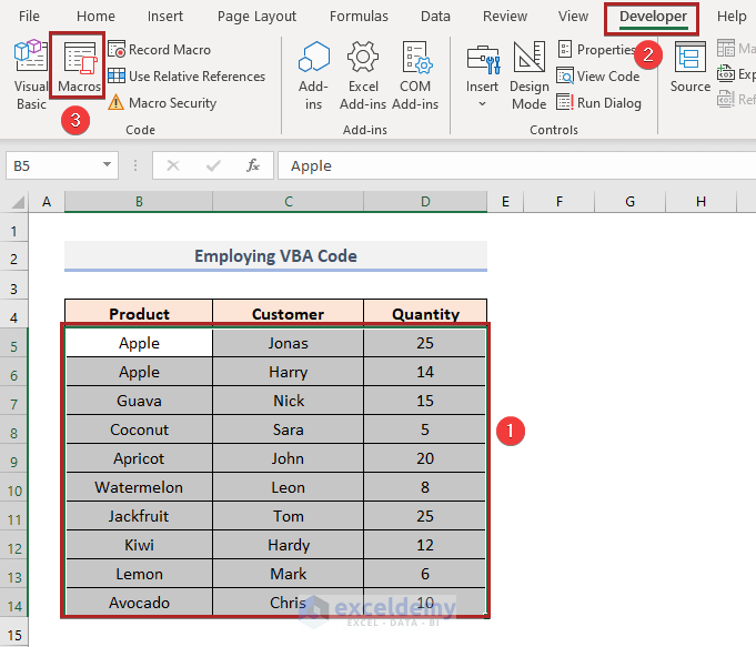
- Go back to the sheet and select the dataset.
- Go to the Developer Tab.
- Select Macros in Code.
- In the Macro wizard, select Alternate_Row_Color (created in the previous step).
- Click Run.
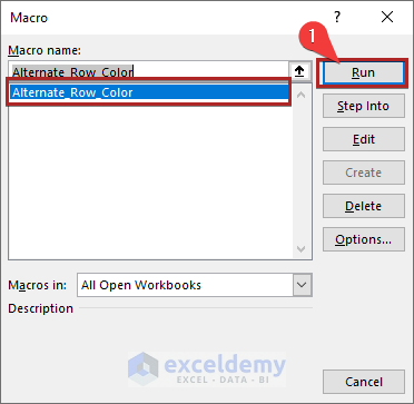
This is the output.
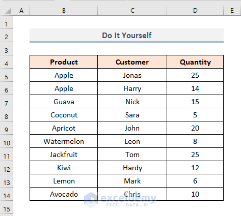
Practice Section
Practice here.
Download Practice Workbook
Download the Excel workbook and practice.
Related Articles
<< Go Back to Highlight Row | Highlight in Excel | Learn Excel
Get FREE Advanced Excel Exercises with Solutions!
