Dataset Overview
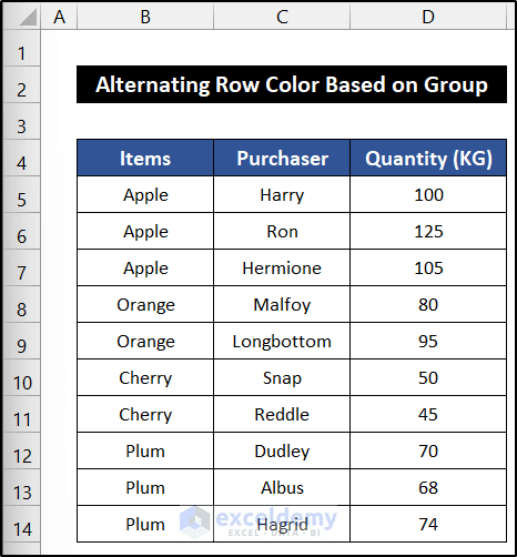
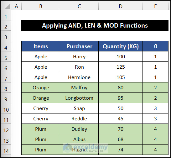
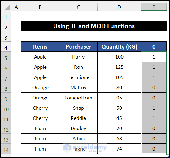
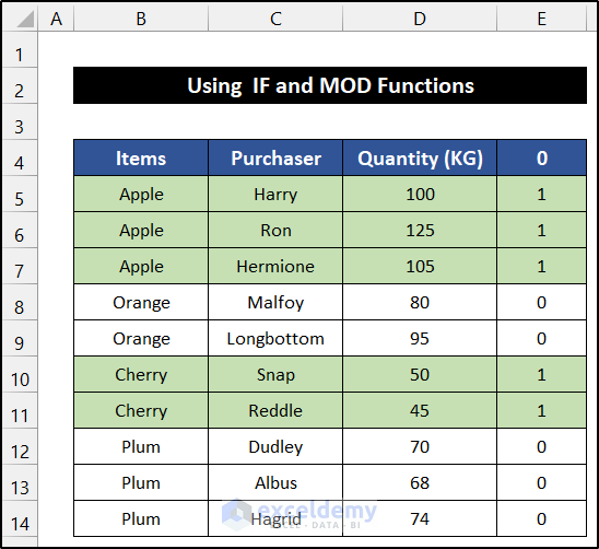
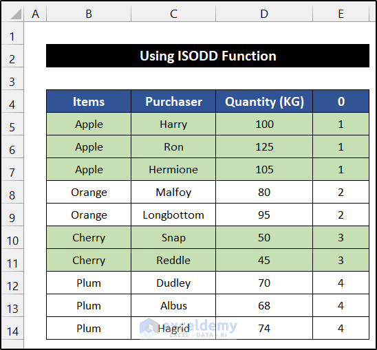
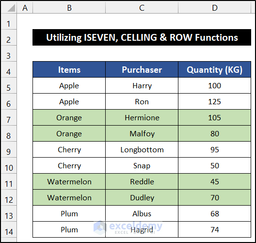
To demonstrate these methods, let’s consider a dataset of 10 fruit consumers. The fruit item names are in column B, and the purchaser names and quantities are in columns C and D, respectively. Our dataset spans the range of cells B5:D14. In each method, we’ll apply conditional formatting to change the cell colors.
Method 1 – Combining AND with LEN and MOD Functions
Steps:
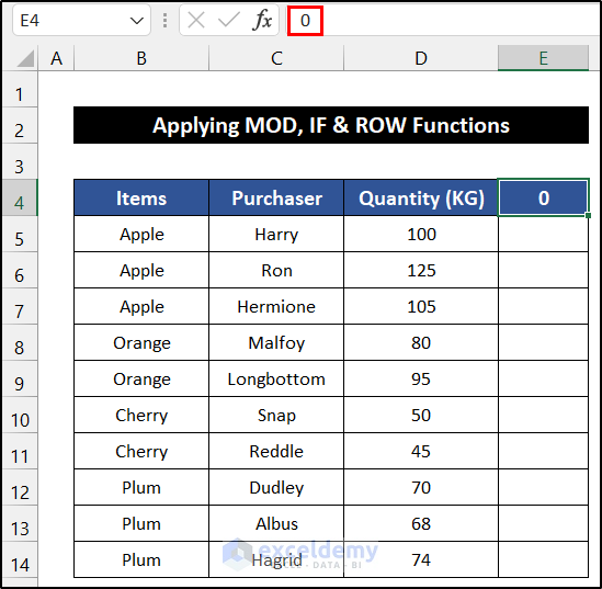
- Select cell E4 and enter “0.”
- Press Enter.

- Select cell E5 and enter the following formula:
=IF(B5=B4,E4,E4+1)
- Press Enter.
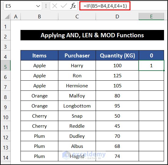
- Double-click the Fill Handle icon to copy the formula down to cell E14.

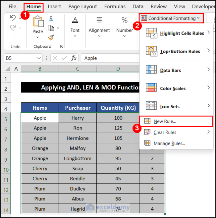
- Select the range of cells B5:E14.
- In the Home tab, click the drop-down arrow of the Conditional Formatting and select the New Rules option from the Styles group.
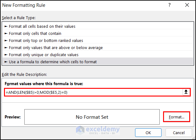
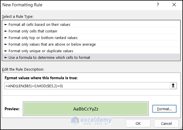
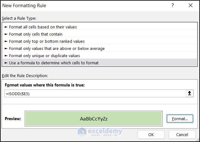
- In the New Formatting Rule dialog box, enter the following formula under Format values where this formula is true:
=AND(LEN($B5)>0,MOD($E5,2)=0)
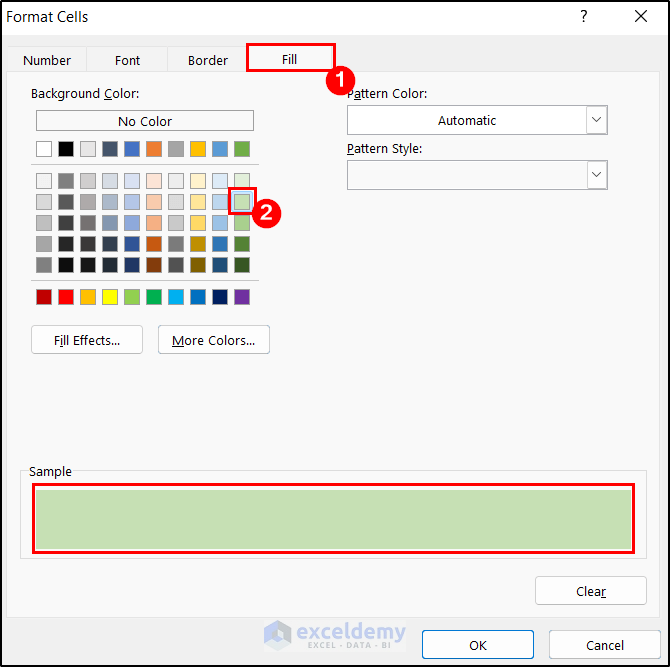
- Click the Format button.
- In the Format Cells dialog box, choose a color (e.g., Green, Accent 6, Lighter 60%) to make the rows distinguishable.
- Click OK.
- Click OK to close the New Formatting Rule dialog box.
- You’ll see the alternating groups of the datasets now shows the selected color.
Breakdown of the Formula
We are breaking down the formula in cell E5.
LEN($B5): This function counts the length of the cell value. In this case, the value is 5.
MOD($E5,2): This function divides the value of cell E5 by 2 and shows the value of the remainder. Here, the result is 1.
AND(LEN($B5)>0,MOD($E5,2)=0): In this formula, the AND function check whether the value of the LEN function is greater than 5 and the result of the MOD function is equal to 0. If both logics are True, the row will show our selected color. Otherwise, it shows as usual.
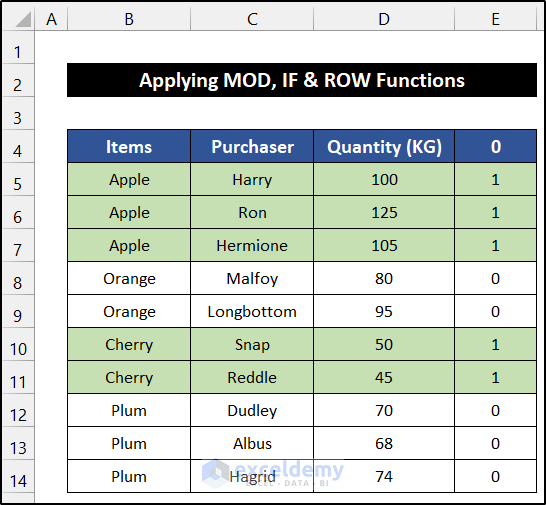
Method 2 – Applying MOD, IF and ROW Functions
Steps:
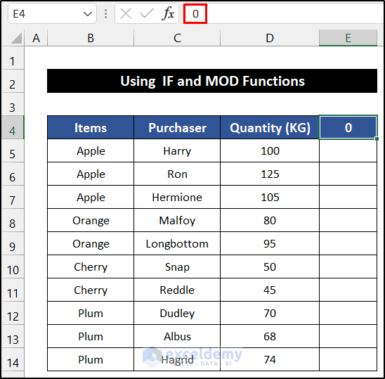
- Select cell E4 and enter “0.”
- Press Enter.
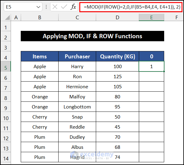
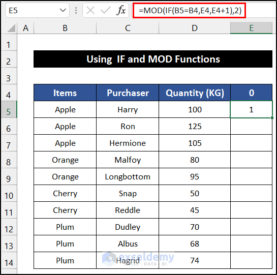
- Select cell E5 and enter the following formula:
=MOD(IF(ROW()=2,0,IF(B5=B4,E4,E4+1)),2)
- Press Enter.
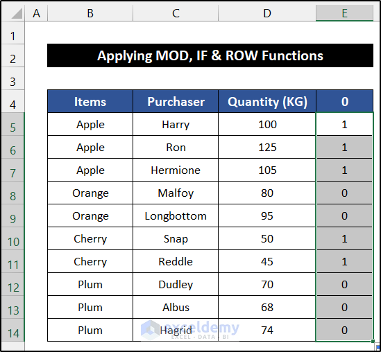
- Double-click the Fill Handle icon to copy the formula down to cell E14.
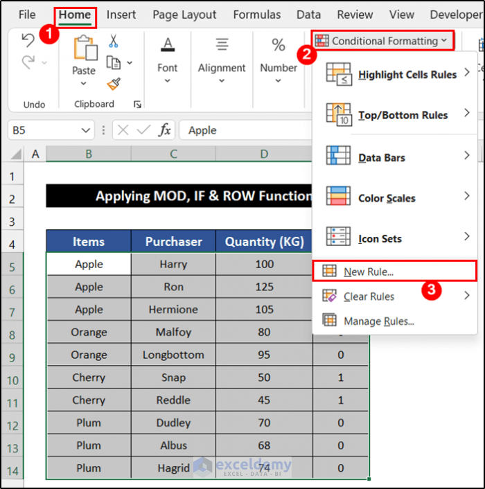
- Select the range of cells B5:E14.
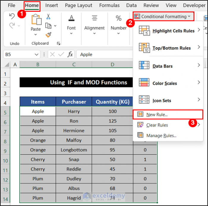
- In the Home tab, click the drop-down arrow of the Conditional Formatting and select the New Rules option from the Styles group.
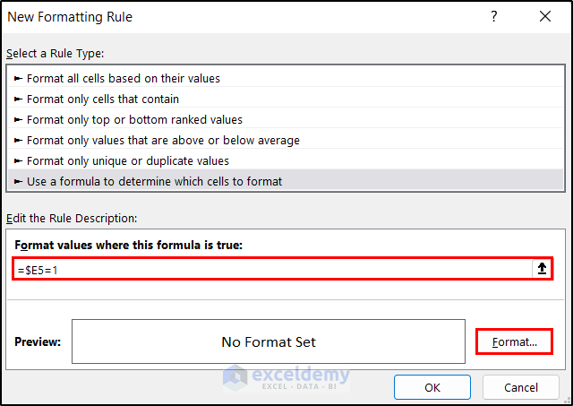
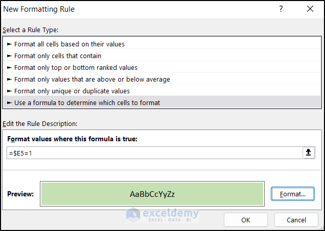
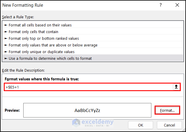
- In the New Formatting Rule dialog box, enter the following formula under Format values where this formula is true:
=$E5=1
- Click the Format button.
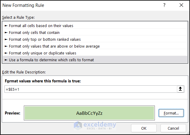
- In the Format Cells dialog box, choose a color (e.g., Green, Accent 6, Lighter 60%) for the alternating rows.
- Click OK.
- Click OK to close the New Formatting Rule dialog box.
- The alternating groups of the datasets will now display the selected color as expected.
Breakdown of the Formula
We are breaking down the formula in cell E5.
ROW(): This function returns the row number. In this case, the value is 5.
IF(B5=B4,E4,E4+1): The IF function checks the value of cell B5 with B4. If both values match each other, the function returns the value of cell E4. Otherwise, it will add 1 with the value of cell E4 and return that.
IF(ROW()=2,0,IF(B5=B4,E4, E4+1)): In this formula, the IF function check whether the row number is equal to 2. If the logic is True, the function returns 0. Or, if the logic is False the function returns the result of the second IF function.
MOD(IF(ROW()=2,0,IF(B5=B4,E4, E4+1)),2): The function will divide the result of the IF function by 2 and show the value of the remainder.
Method 3 – Combining MOD and IF Functions
Steps:
- Select cell E4 and enter “0.”
- Press Enter.
- Select cell E5 and enter the following formula:
=MOD(IF(B5=B4,E4,E4+1),2)
- Press Enter.
- Double-click the Fill Handle icon to copy the formula down to cell E14.
- Select the range of cells B5:E14.
- In the Home tab, click the drop-down arrow of the Conditional Formatting and select the New Rules option from the Styles group.
- In the New Formatting Rule dialog box, enter the following formula under Format values where this formula is true:
=$E5=1
- Click the Format button.
- In the Format Cells dialog box, choose a color (e.g., Green, Accent 6, Lighter 60%) to make the rows distinguishable.
- Click OK.
- Click OK to close the New Formatting Rule dialog box.
- You’ll see the alternating groups of the datasets now shows the selected color.
Breakdown of the Formula
We are breaking down the formula in cell E5.
IF(B5=B4,E4,E4+1): The IF function checks the value of cell B5 with B4. If both values match each other, the function returns the value of cell E4. Otherwise, it will add 1 with the value of cell E4 and return that.
MOD(IF(B5=B4,E4,E4+1),2): The function will divide the result of the IF function by 2 and show the value of the remainder.
Method 4 – Applying ISODD Function
Steps:
- Select cell E4 and enter “0.”
- Press Enter.

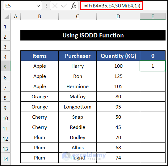
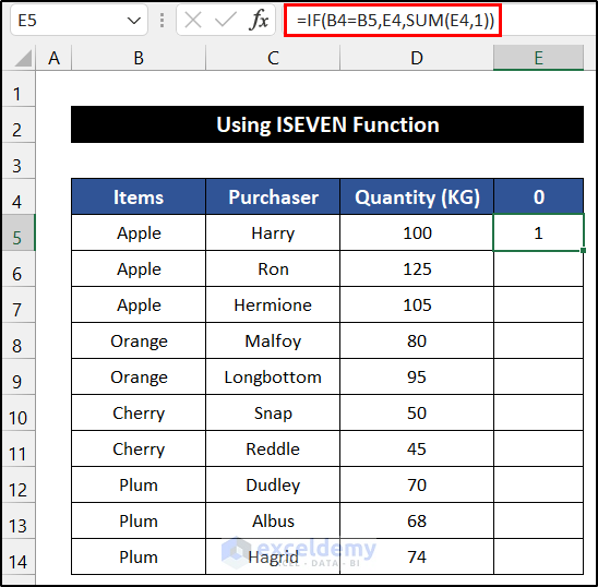
- Select cell E5 and enter the following formula:
=IF(B4=B5,E4,SUM(E4,1))
- Press Enter.
- Double-click the Fill Handle icon to copy the formula down to cell E14.
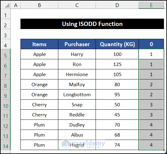
- Select the range of cells B5:E14.
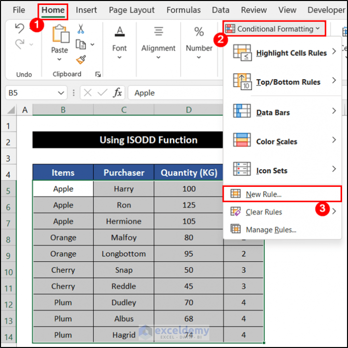
- In the Home tab, click on the drop-down arrow of the Conditional Formatting and select the New Rules option from the Styles group.
- In the New Formatting Rule dialog box, enter the following formula under Format values where this formula is true:
=ISODD($E5)
- Click the Format button.

- In the Format Cells dialog box, choose a color (e.g., Green, Accent 6, Lighter 60%) for the alternating rows.
- Click OK.
- Click OK to close the New Formatting Rule dialog box.
- The alternating groups of the datasets will now display the selected color as expected.
Breakdown of the Formula
We are breaking down the formula in cell E5.
SUM(E4,1): The function will add 1 with the value of cell E4. For this cell, the function returns 1.
IF(B4=B5,E4,SUM(E4,1)): The IF function checks the value of cell B5 with B4. If both values match each other, the function returns the value of cell E4. On the other hand, if the logic is False, it returns the result of the SUM function.
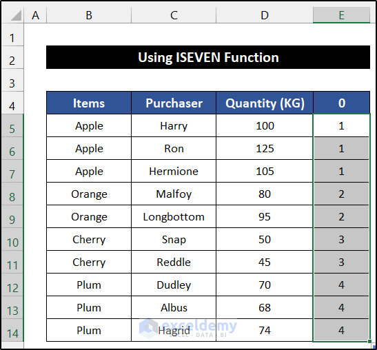
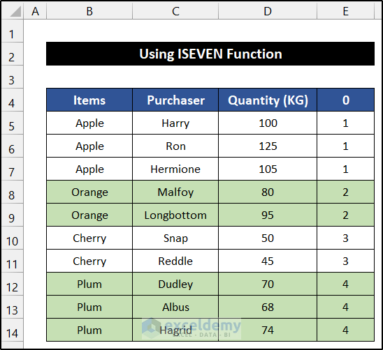
Method 5 – Using ISEVEN Function
Steps:
- Select cell E4 and enter “0.”
- Press Enter.

- Select cell E5 and enter the following formula:
=IF(B4=B5,E4,SUM(E4,1))
- Press Enter.
- Double-click the Fill Handle icon to copy the formula down to cell E14.
- Select the range of cells B5:E14.
- In the Home tab, click on the drop-down arrow of the Conditional Formatting and select the New Rules option from the Styles group.
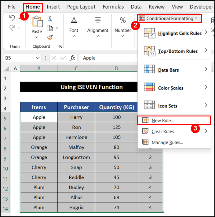
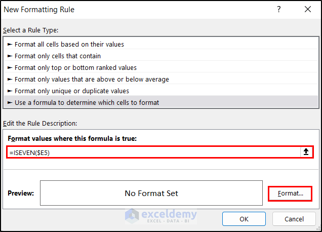
- In the New Formatting Rule dialog box, enter the following formula under Format values where this formula is true:
=ISEVEN($E5)
- Click the Format button.
- In the Format Cells dialog box, choose a color (e.g., Green, Accent 6, Lighter 60%) for the alternating rows.
- Click OK.
- Click OK to close the New Formatting Rule dialog box.

- The alternating groups of the datasets will now display the selected color as expected.
Breakdown of the Formula
We are breaking down the formula in cell E5.
SUM(E4,1): The function will add 1 with the value of cell E4. For this cell, the function returns 1.
IF(B4=B5,E4,SUM(E4,1)): The IF function checks the value of cell B5 with B4. If both values match each other, the function returns the value of cell E4. On the other hand, if the logic is False, it returns the result of the SUM function.
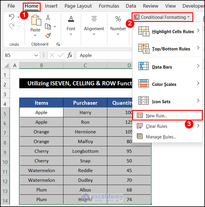
Method 6 – Utilizing ISEVEN, CELLING and ROW Functions
Steps:
- Select the range of cells B5:E14.
- In the Home tab, click on the drop-down arrow of the Conditional Formatting and select the New Rules option from the Styles group.
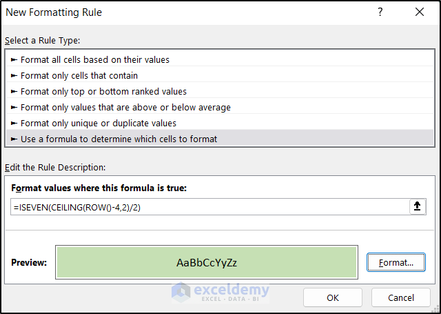
- In the New Formatting Rule dialog box, enter the following formula under Format values where this formula is true:
=ISEVEN(CEILING(ROW()-4,2)/2)
- Click the Format button.

- In the Format Cells dialog box, choose a color (e.g., Green, Accent 6, Lighter 60%) to make the rows distinguishable.
- Click OK to close the Format Cells dialog box.
- Cick OK to close the New Formatting Rule dialog box.
- You’ll get the alternating groups of the datasets showing the selected color.
Breakdown of the Formula
We are breaking down the formula for row 5.
ROW(): This function returns the row number. In this case, the value is 5.
CEILING(ROW()-4,2): This function deducts 4 from the result of the ROW function and then multiplies the value with 2. Here, the result is 2.
ISEVEN(CEILING(ROW()-4,2)/2): In this formula, the ISEVEN function checks whether the division value of the result of the CEILING function and 2. If the value is even, the row will show our selected color. Otherwise, it shows as usual.
Things You Should Know
Keep in mind that we enter the formula directly in the conditional formatting rule box without performing any numerical grouping. So, ensure that the number of group entities remains equal for accurate results.
Download Practice Workbook
You can download the practice workbook from here:
Related Articles
- How to Color Alternate Row Based on Cell Value in Excel
- How to Alternate Row Colors in Excel Without Table
<< Go Back to Highlight Row | Highlight in Excel | Learn Excel
Get FREE Advanced Excel Exercises with Solutions!
