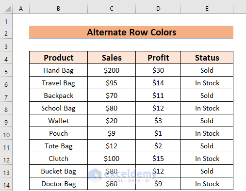
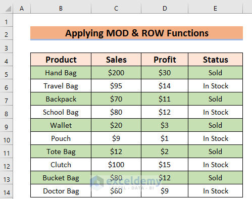
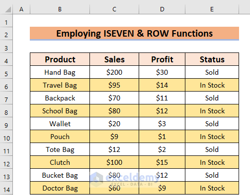
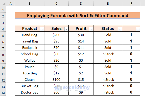
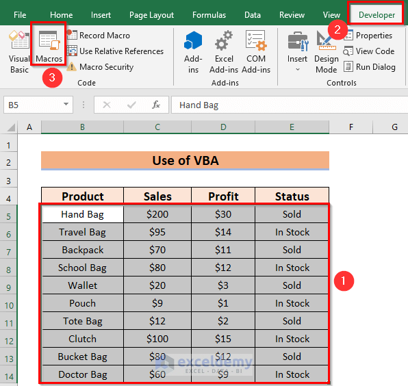
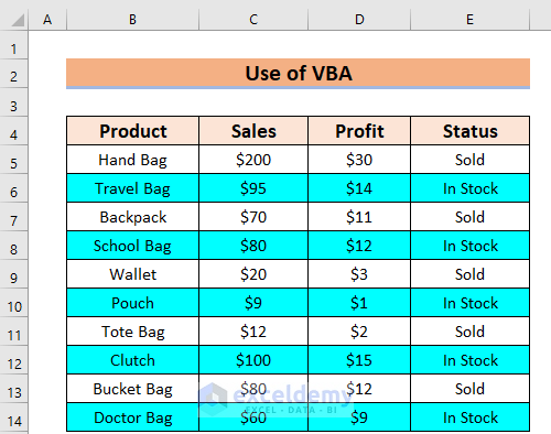
How to Alternate Row Colors in Excel Without a Table (5 Methods)

The sample dataset below has 4 columns: Product, Sales, Profit, and Status.

How to Alternate Row Colors in Excel Without Table

Method 1 – Using the Fill Color Option to Alternate Row Colors

Steps:

Select the Rows you want to color. Here, I have selected Rows 6, 8, 10, 12, and 14.

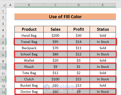
Go to the Home tab.
From the Fill Color feature >> choose any of the colors. Here, I have chosen Green, Accent 6, Lighter 60%. In this case, try to choose a light color because the dark color may hide the inputted data. Then, you may need to change the Font Color.

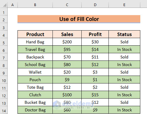
You will see the result with alternate Row colors.

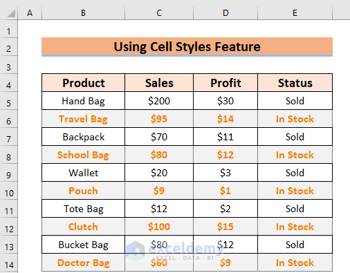
Method 2 – Applying the Cell Styles Feature to Alternate Row Colors

Steps:

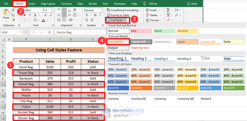
Select the Rows you want to color. Here, I have selected Rows 6, 8, 10, 12, and 14.
From the Home tab >> go to the Cell Styles feature.
Choose your preferred colors or styles. Here, I have chosen the Calculation.

You will see the following result with alternate Row colors.

Method 3 – Applying Conditional Formatting with Formula to Alternate Row Colors

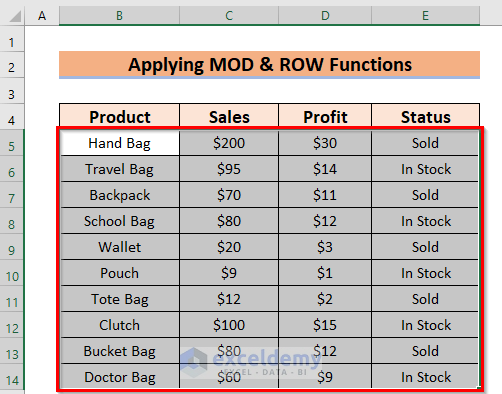
3.1. Use of MOD and ROW Functions

Steps:

Select the data you want to apply the Conditional Formatting to alternate the row colors. Here, I have selected the data range B5:E14.

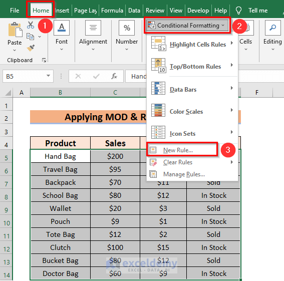
From the Home tab >> go to the Conditional Formatting command.
Choose the New Rule option to apply the formula.

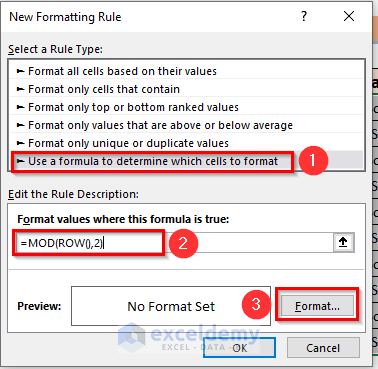
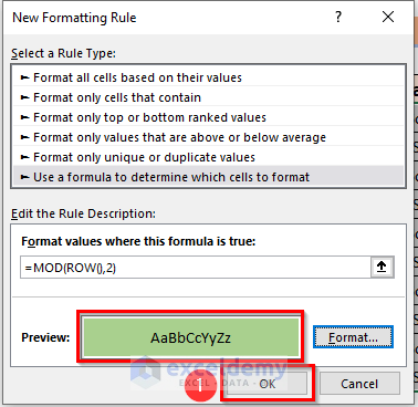
A dialog box named New Formatting Rule will appear.

Select Use a formula to determine which cells to format.
Enter the following formula in the Format values where this formula is true: box.

=MOD(ROW(),2)

Go to the Format menu.

Formula Breakdown

Here, the ROW function will count the number of Rows.
The MOD function will return the remainder after division.
So, MOD(ROW(),2)–> Becomes 1 or 0 because the divisor is 2.
Finally, if the Output is 0 then there will be no fill color.

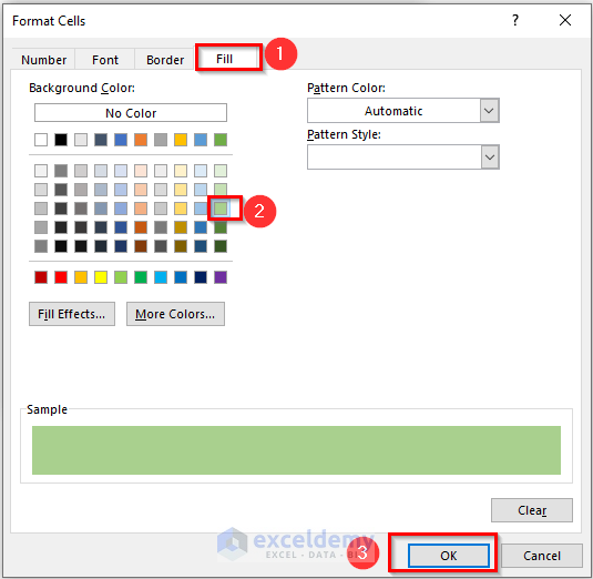
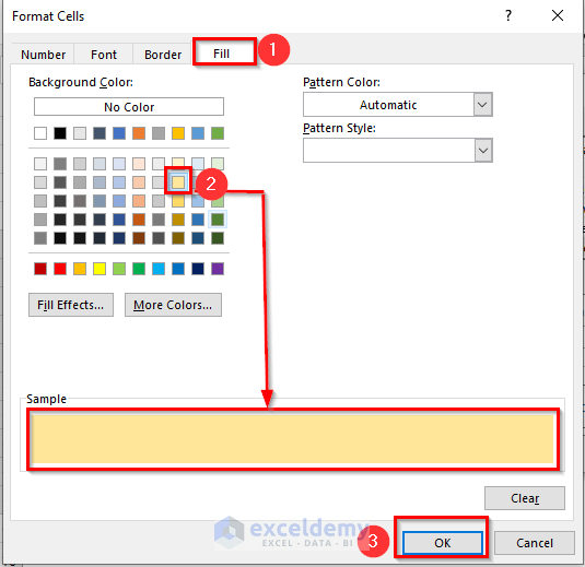
A dialog box named Format Cells will appear.

From the Fill option >>choose any of the colors. Here, I have chosen Green, Accent 6, Lighter 40%. In this case, try to choose any light color because the dark color may hide the inputted data. Then, you may need to change the Font Color.
Press OK to apply the formation.

Press OK on the New Formatting Rule dialog box. Here, you can see the sample instantly in the Preview box.

You will get the result with alternate Row colors.

3.2. Use of ISEVEN and ROW Functions to Alternate Row Colors in Excel

Follow method-3.1 to open the New Formatting Rule window.
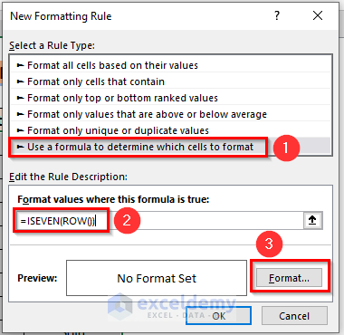
From that dialog box >> select Use a formula to determine which cells to format.
Enter the following formula in the Format values where this formula is true: box.

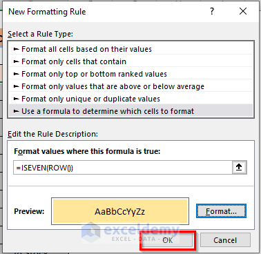
=ISEVEN(ROW())

Go to the Format menu.

Formula Breakdown

Here, the ISEVEN function will return True if the value is an even number.
The ROW function will count the number of Rows.
So, if the Row number is odd then the ISEVEN function will return FALSE. As a result there will be no fill color.

A dialog box named Format Cells will appear.

From the Fill option >> choose any of the colors. Here, I have chosen Gold, Accent 4, Lighter 60%. Also, you can see the formation in the Sample box below.
Press OK to apply the formation.

Press OK on the New Formatting Rule dialog box. Here, you can see the sample instantly in the Preview box.

You will see the result with alternate Row colors.

Method 4 – Using an Excel Formula with Sort & Filter Command to Alternate Row Colors

Steps:

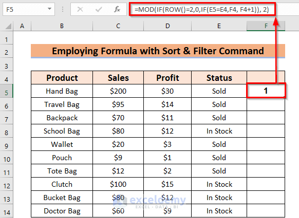
Select a cell where you want to keep the output. I have selected cell F5.
Enter the corresponding formula in cell F5:

=MOD(IF(ROW()=2,0,IF(E5=E4,F4, F4+1)), 2)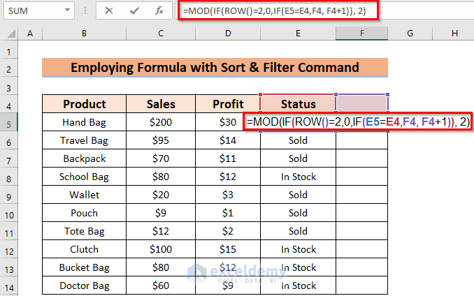

Formula Breakdown

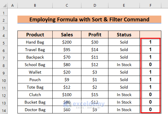
Here, IF(E5=E4,F4, F4+1)–> This is a logical test where if the value of E5 cell is equal to E4 cell then it will return the value of F4 cell otherwise it will give 1 increment with F4 cell value.
- Output: 1
Then, the ROW() function will count the number of Rows.
- Output: 5
IF(5=2,0,1)–> This logical test says that if 5 is equal to 2 then it will return 0 otherwise it will return 1.
- Output: 1
The MOD function will return the remainder after division.
Finally, MOD(1,2)–> becomes.
- Output: 1

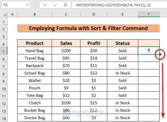
Press ENTER to get the result.

Drag the Fill Handle icon to AutoFill the corresponding data in the rest of the cells F6:F14.

You will see the following result.

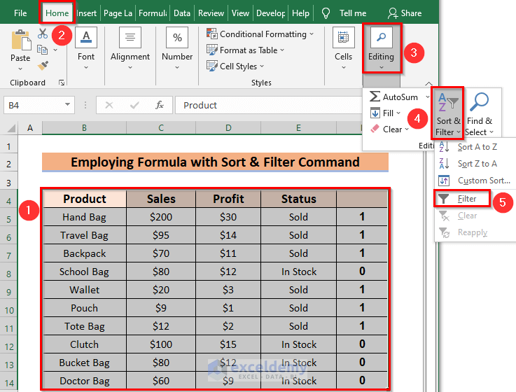
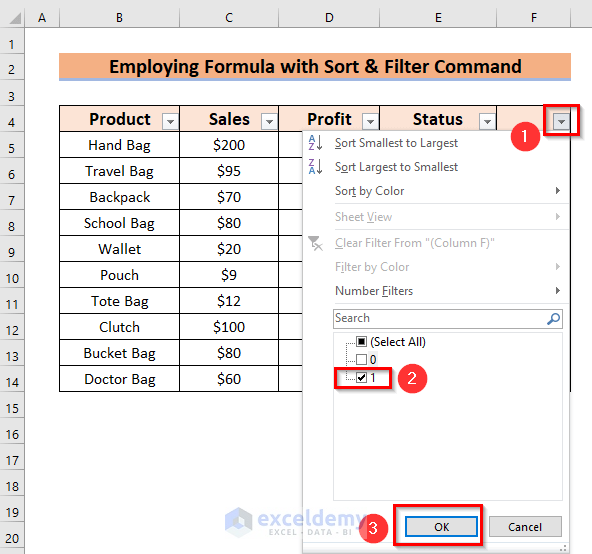
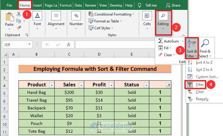
Select the data range. Here, I have selected B4:F14.
From the Home ribbon >> go to the Editing tab.
From the Sort & Filter feature >> choose the Filter option. Here, you can apply the Keyboard technique CTRL+SHIFT+L.

You will see the following situation.

Click on the Drop-Down Arrow on the F column.
Select 1 and uncheck 0.
Press OK.

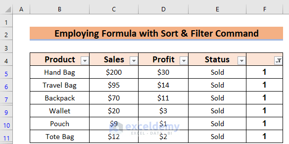
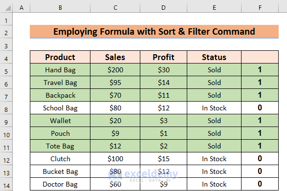
You will see the following filtered output.

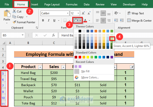
Select the filtered data.
Go to the Home tab.
From the Fill Color feature >> choose any of the colors. Here, I have chosen Green, Accent 6, Lighter 60%.

To remove the Filter feature, from the Home ribbon >> go to the Editing tab.
From the Sort & Filter feature >> choose again the Filter option.
Otherwise, you can press CTRL+SHIFT+L to remove the Filter feature.

You will see the result with the same Row colors for the same Status.

Method 5 – Applying VBA Code to Alternate Row Colors

Steps:

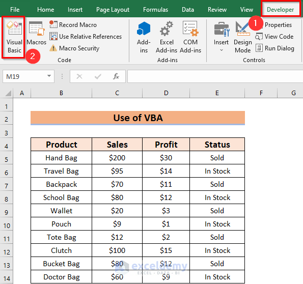
Choose the Developer tab >> select Visual Basic.

From the Insert tab >> select Module.

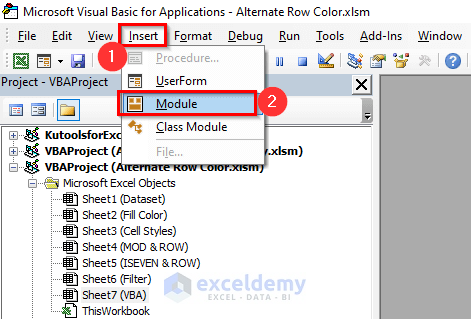
Enter the following Code in the Module:

Sub ChangeRowColors()
Dim range As range
Dim chr As Long
Dim NoColor As Long
Dim Colored As Long
'I will Define Color as Input
  NoColor = vbWhite
  Colored = RGB(0, 255, 255)
'Select a range as variable
  Set range = Selection
'You should select more than 1 Row
  If range.Rows.Count = 1 Then Exit Sub
'Loop for Color Changing
  For chr = 1 To range.Rows.Count
    If chr Mod 2 = 0 Then
      range.Rows(chr).Interior.Color = Colored 'Even Row
    Else
      range.Rows(chr).Interior.Color = NoColor 'Odd Row
    End If
  Next chr
End Sub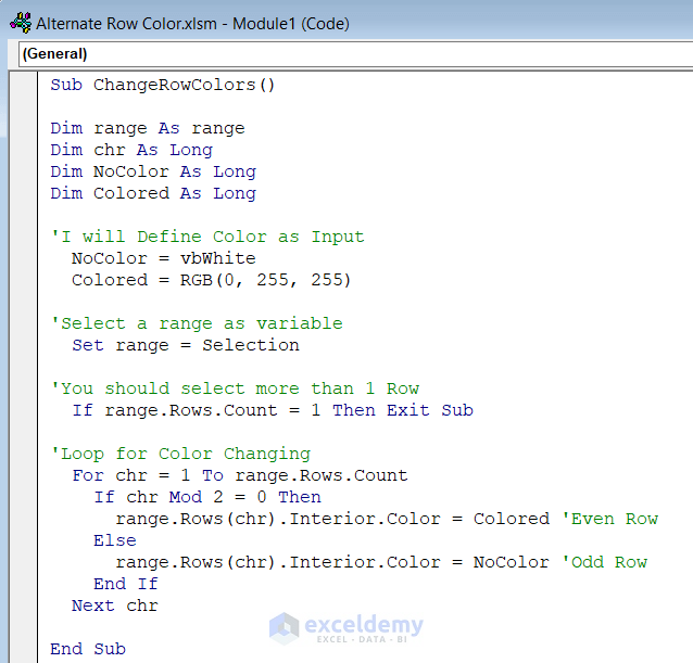

Code Breakdown

Here, I have created a Sub Procedure named ChangeRowColors.
Next, declare some variables range as Range to call the range; chr as Long; NoColor as Long; Colored as Long.
Here, RGB (0, 255, 255) is a light color called Aqua.
Then, the Selection property will select the range from the sheet.
After that, I used a For Each Loop to put Color in each alternate selected Row using a VBA IF Statement with a logical test.

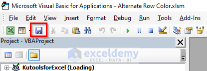
Save the code then go back to Excel File.

Select the range B5:E14.
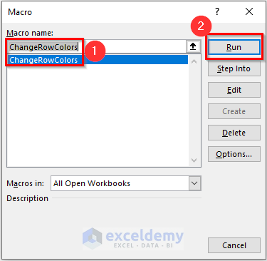
From the Developer tab >> select Macros.

Select Macro (ChangeRowColors) and click on Run.

You will see the result with alternate Row colors.

Things to Remember

When you have lots of data, you should use method 3 (Conditional Formatting) or method 5 (VBA Code). This will save you time alternating Row colors.
In the case of a tiny dataset, you can easily use method 1 (Fill Color) or method 2 (Cell Styles).
Furthermore, when you want to color similar data or sort something, you should use method 4 (Sort & Filter).

How to Alternate Row Colors in Excel Without a Table (5 Methods)

Method 1 – Using the Fill Color Option to Alternate Row Colors

Method 2 – Applying the Cell Styles Feature to Alternate Row Colors

Method 3 – Applying Conditional Formatting with Formula to Alternate Row Colors

3.1. Use of MOD and ROW Functions

3.2. Use of ISEVEN and ROW Functions to Alternate Row Colors in Excel

Method 4 – Using an Excel Formula with Sort & Filter Command to Alternate Row Colors

Method 5 – Applying VBA Code to Alternate Row Colors

Things to Remember

Related Articles

Leave a reply Cancel reply