Creating Interactive KPI Scorecards in Google Sheets

KPI stands for key performance indicators, and refers to a measurement of a set of targets against some goalpost. KPI scorecards are essential in tracking business goals, trends, and overall performance. Google Sheets offers powerful tools to create interactive KPI scorecards. KPI scorecards will allow you to visualize performance to take further initiatives.

In this article, we will show how to create interactive KPI scorecards in Google Sheets.

Let’s consider sample sales KPI data to walk you through the steps to create a dynamic KPI scorecard with conditional formatting, charts, and interactivity.

Step 1: Set Up Your Data

Identify and list the KPI categories you want to track in a scorecard. It can be sales growth, revenue, customer retention, satisfaction, etc.

We are listing some required data and KPIs as follows:

• Date
• Department
• KPI Name
• Target Value
• Actual Value
• Progress (%)
• Status

You can use Google Sheets formulas to calculate progress and status.

Progress (%):

• Select cell F2 and insert the following formula.
• Drag the formula down to the progress percentage for each row.

Formula:

=IF(E2="","", E2/D2)

This formula will divide the actual value by the target value to return the progress percentage. Then select Percentage (%) to show the Progress (%).

Output:

Status:

• Select cell G2 and insert the following formula.
• Drag the formula down to determine the status of each row.

Formula:

=IF(F2>=100%, "On Track", IF(F2>=90%, "Warning", "At Risk"))

This formula will check the progress percentage and then return the KPI status.

Output:

Step 2: Apply Conditional Formatting

Let’s use the Conditional Formatting to highlight Progress (%) and Status.

Highlight Status Column:

• Select the Status column.
• Go to the Format tab >> select Conditional Formatting.
• Format rules: Text contains.
  • On Track: Green
  • Warning: Yellow
  • At Risk: Red
• Click Done.

Status are filled with respective colors.

Color Gradient to Progress (%):

• Select the Progress (%) column.
• Go to the Format tab >> select Conditional Formatting.
• Select Colour scale to apply a gradient color scale.
• Format rules:
  • Minpoint: 0%; Color: Red
  • Midpoint: 90%; Color: Yellow
  • Maxpoint: 100%; Color: Green
• Click Done.

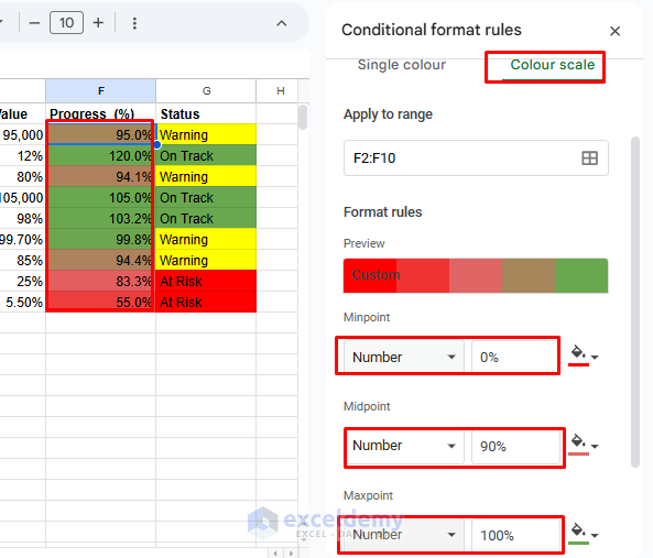
Progress percentages are filled with gradient colors.

Step 3: Add Filters and Dropdowns for Dynamic Interaction

Dropdown for Date Filtering:

• Select cell I2.
• Go to the Data tab >> select Data Validation.
• In Criteria >> select Drop-down(from a range)
• Select data range: A2:A10
• Click Done.

You will get a dropdown to select specific dates.

Dynamic Dropdown for Department:

• Select an empty cell and insert the following formula.

Formula:

=UNIQUE(FILTER(B2:B10, A2:A10=I2))

This formula will filter the unique department name based on the date of the I2 cell.

Let’s create a dropdown for department selection (e.g., K1).

• Select cell J2.
• Go to the Data tab >> select Data Validation.
• In Criteria >> select Drop-down(from a range)
• Select data range: P3:P4 (It’s the list where we applied the FILTER and UNIQUE formula).
• Click Done.

You will get a dependent drop-down list. Based on the Date drop-down you will get the department list.

After creating the drop-down list you can hide the department list (P3:P4).

FILTER Function to Display Data for the Selected Date:

• Select data from the Drop-down list.
• Select cell I4 and insert the following formula.

Formula:

=FILTER(A2:G10, A2:A10=I2)

This will filter the KPI data based on the specific date of the drop-down list.

Filter based on the selected Date and Department:

• Select a Date and Department name from the drop-down lists.
• Select cell I6 and insert the following formula.

Formula:

=FILTER(A2:G10, A2:A10=I2, B2:B10=J2)

This formula will filter the KPI data based on the date and department.

 Step 4: Add Interactive Charts and Visuals

Insert Progress Bars:

You can use the SPARKLINE function to create visual progress bars for the Progress (%) column.

• Select cell Q1 and insert the following formula.
• Copy the formula down for all progress values.

=SPARKLINE(F2, {"charttype", "bar"; "max", MAX($F$2:$F$10); "min", 0; "color1", "#4CAF50"})

This formula will create a bar chart based on the progress bar maximum value.

Output:

Create a Line Chart for Performance Over Time:

• Select Date and Progress (%) columns.
• Go to the Insert tab >> select Chart.

• In the Chart Editor >> from Chart Type >> select Line Chart.

Add a Column Chart for Status:

• Select the Status column.
• Go to the Insert tab >> select Chart.
• In the Chart Editor >> from Chart Type >> select Bar Chart.

Add a Pie Chart for Status Percentage:

• Select the Status column.
• Go to the Insert tab >> select Chart.
• In the Chart Editor >> from Chart Type >> select Pie Chart.

Add a Scorecard for Minimum and Maximum Progress:

• Select the Progress (%) column.
• Go to the Insert tab >> select Chart.
• In the Chart Editor >> from Chart Type >> select Scorecard.
• Click on Aggregate >> select Min to show the minimum progress.

• Click on Aggregate >> select Max to show the maximum progress.

Add Custom Icons (Optional):

You can use symbols (e.g., ⬆ for “up” and ⬇ for “down”) to represent trends.

• Insert the following formula to display trend indicators.

Formula:

=IF(F2>=100%, "", IF(F2>=90%, "", ""))

This formula will display symbols based on the progress (%)

Output:

Step 5: Use Slicers for User Interactivity

Add a Slicer:

• Select the data range.
• Go to the Data tab >> select Add a slicer.

• Select the Date column.

KPI Dashboard:

Organize all the features, charts, and values in a structured way to give a professional look. Position the charts and dropdowns to create a neat, interactive dashboard layout.

Conclusion

By following the above steps, you can create an interactive KPI scorecard in Google Sheets. This will help you to track and visualize performance progress in real-time. We used dynamic charts to create a visually appealing scorecard with progress bars, conditional formatting, and charts. You can use these types of scorecards for personal projects or corporate goals, which makes performance tracking simple and effective.