Method 1 – Create a Cross Functional Flowchart in Excel with Microsoft Visio
STEPS:
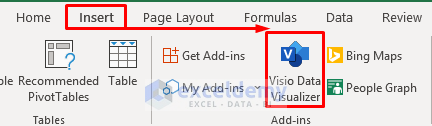
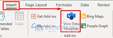
- Create a new sheet, go to the Insert tab, and select Visio Data Visualizer.
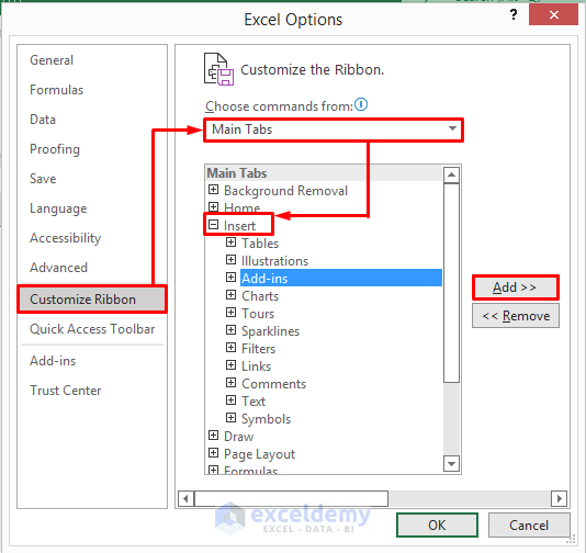
- If you don’t find it inside the Insert tab, you need to add it. To do so, click on File >> Options. It will open the Excel Options window.
- In the Excel Options window, select Customize Ribbon >> Main Tabs >> Insert >> Add-ins.
- Click Add and OK to proceed.
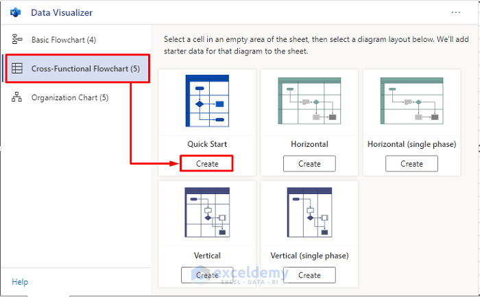
- After selecting Visio Data Visualizer, the Data Visualizer window will appear.
- Go to the Cross-Functional Flowchart tab and click on Create. Choose the chart according to your needs. We chose the Quick Start flowchart here.
- The cross-functional flowchart and a table will appear on the sheet.
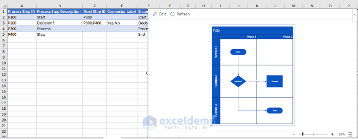
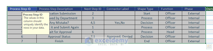
- You need to enter the information in the table to create a chart.
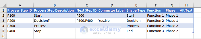
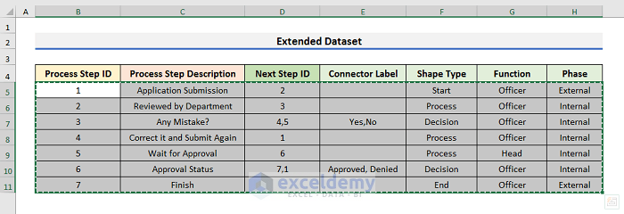
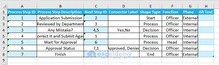
- Copy the Extended Dataset without the headers.

- Go to the sheet where the Visio table is located and select Cell A2.
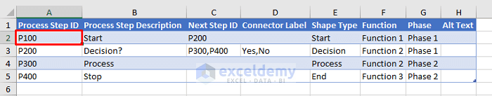
- Press Ctrl + V to paste the information.
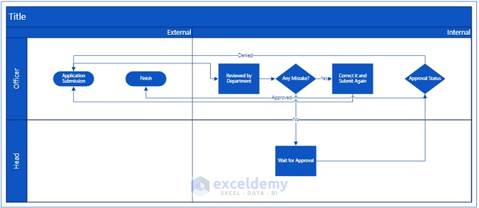
- Click the Refresh icon in the flowchart sheet.
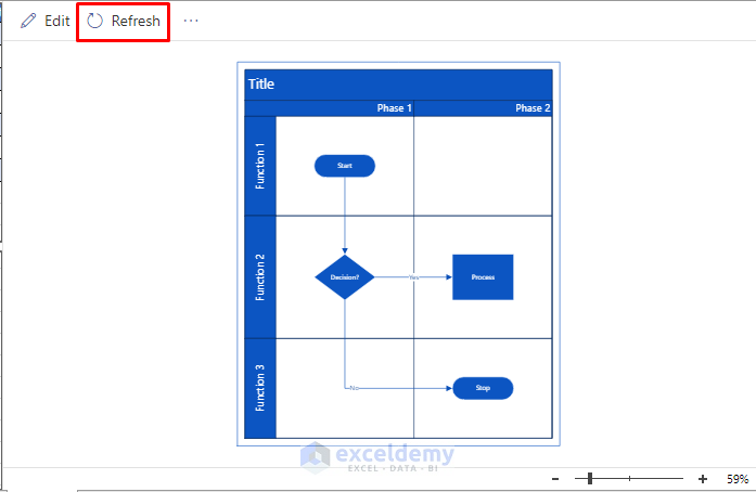
- Get a cross-functional flowchart like the one in the picture below.

Method 2 – Make a Cross Functional Flowchart in Excel Online
STEPS:
- Click on the File tab.
- Click on New and select Charts.
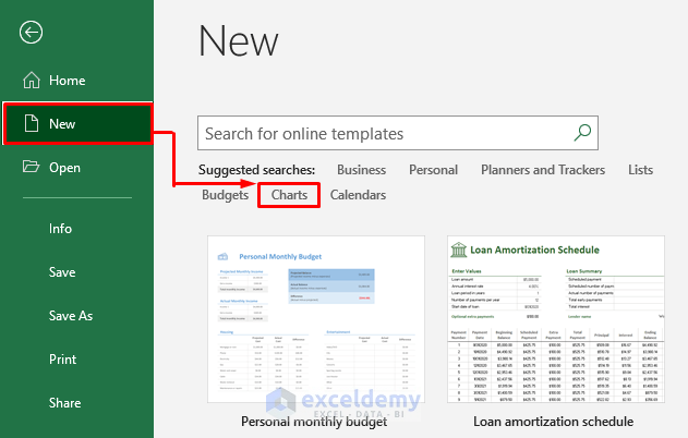
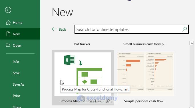
- Scroll down and select Process Map Cross-Functional Flowchart.
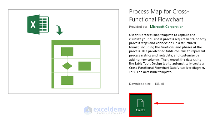
- Click Create.
- A new window will appear with 4 sheets.
- Click the Process Map sheet.
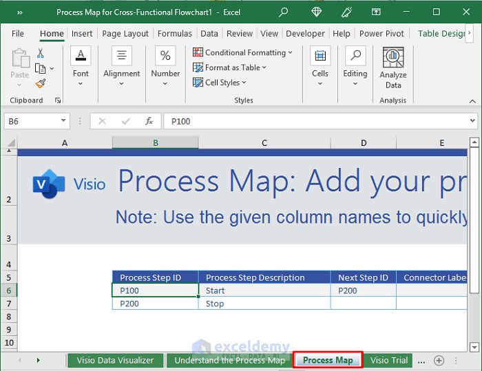
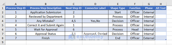
- Copy the Extended Dataset from the old workbook.
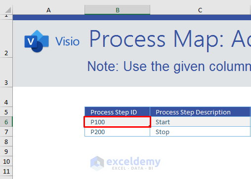
- Select Cell B6 from the Process Map sheet and press Ctrl + V to paste the Extended Dataset.
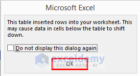
- A message will pop up. Click OK to proceed.
- Select the dataset in the Process Map sheet and copy it.
- Create a new sheet on the same workbook and click on the Visio Data Visualizer icon.
- Press Ctrl + V to paste the copied data.
- Click on Refresh and create the cross-functional flowchart.
Method 3 – Import a Cross Functional Flowchart from Scratch in Excel
STEPS:
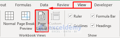
- Navigate to the View tab and select Page Layout.
- Go to the Home tab, click the Format icon, and select Row Height from the drop-down menu.
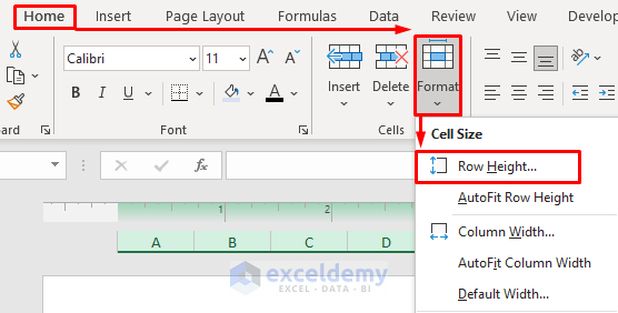
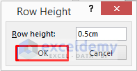
- Set the row height to 0.5 cm and click OK.
- Go to the Home tab, select the Format icon, and then click on the Column Width option.
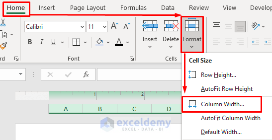
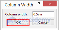
- Set the column width to 0.5cm and click OK to proceed.
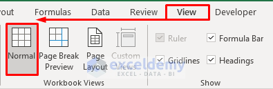
- Go to the View tab and select Normal.
- Select the range A2:AH6.
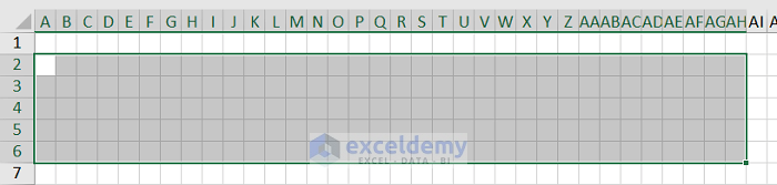
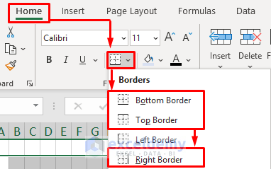
- Go to the Home tab and select Bottom, Top, and Right borders.
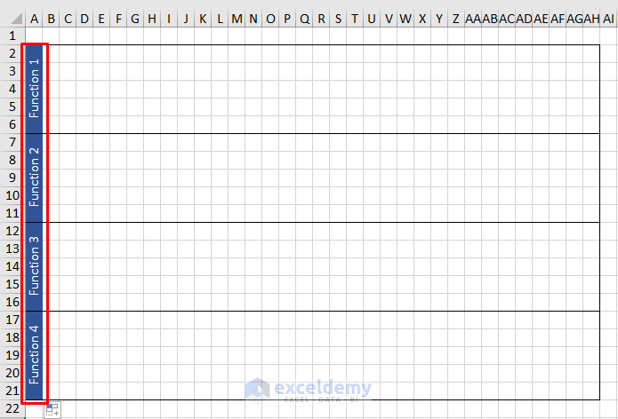
- Select Cell A2 to A6.
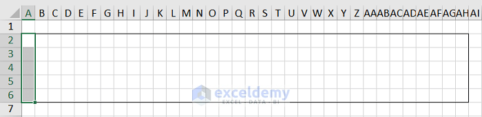
- Click Merge & Center in the Home tab.
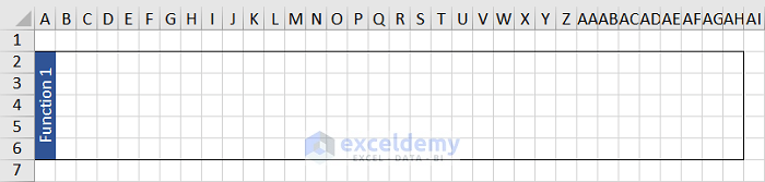
- Type Function 1 inside the merged cell.
- Fill the merged cell with a color from the Font section in the Home tab. You can change the font color if you want.
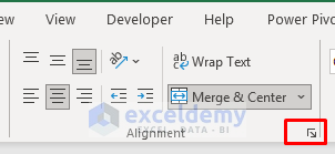
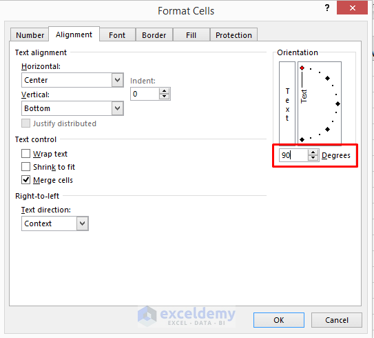
- After completing the previous steps, go to the Alignment section in the Home tab and click the Alignment Settings icon.
- Type 90 in the Orientation section and click OK.
- The sheet will look like the screenshot below.
- Copy the range A2:AH6 and paste it into the below ranges.
- Change the name of the functions to Function 2, Function 3, and Function 4 respectively.
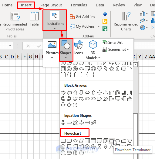
- You need to enter the flowchart shapes.
- Go to the Insert tab and select Illustrations. A drop-down menu will appear.
- Select Shapes and scroll down to Flowchart.
- Select the Terminator icon and insert the shape into the sheet.
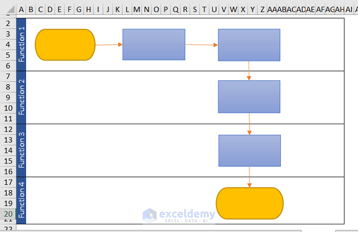
- Follow the same procedure and insert the Rectangular shapes into the sheet.
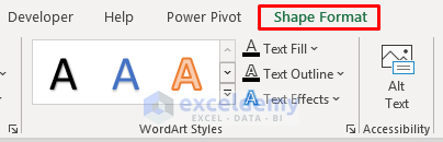
- Click on any shape, and the Shape Format tab will appear on the ribbon.
- Use this tab to apply different styles to the texts inside the shapes.
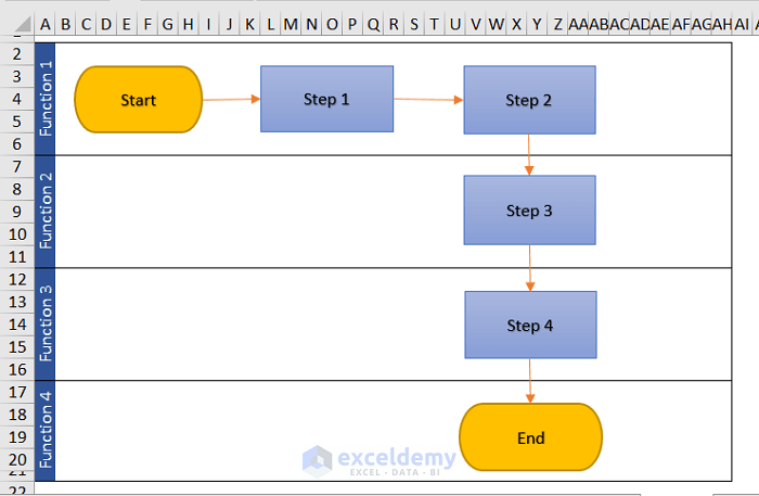
- Type the name of the process and step in each box to make a cross-functional like the one below.
Download the practice book here.
Related Articles
<< Go Back to Flowchart in Excel | Learn Excel
Get FREE Advanced Excel Exercises with Solutions!
