Method 1 – Create a Grid
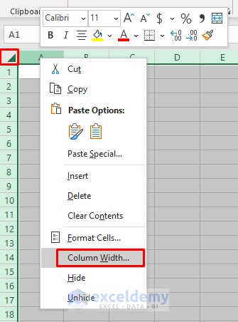
- Click on the upper-left corner (red-colored box) of the spreadsheet.
- Right-click on any of the Columns.
- Get the context menu. Select Column Width.
- The Column Width dialog box will pop out.
- Type 2.14 in the box.
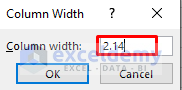
- Press OK.
- See the grid in the worksheet.
Method 2 – Enable Snap
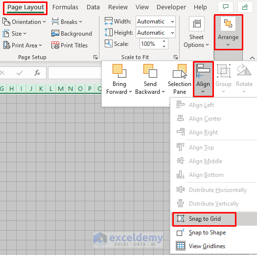
- Go to the Page Layout tab.
- Select Arrange ➤ Align ➤ Snap to Grid.
- The feature gets activated.
Method 3 – Modify Excel Page Layout
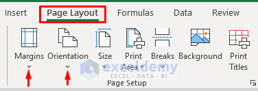
Set the Page as per your choice and requirements. Under the Page Layout tab, you’ll get the Page Setup section. Choose your desired Margin, Orientation, etc. Choose Normal from the Margin drop-down and Portrait from the Orientation drop-down.
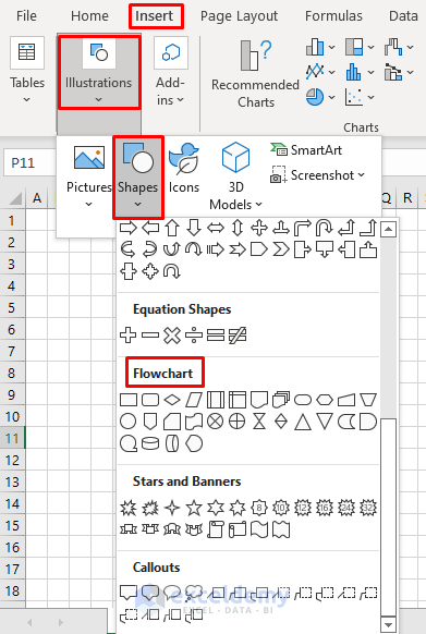
Method 4 – Insert & Edit Flowchart Shapes
- Go to the Insert tab.
- In the Illustrations drop-down, select Shapes.
- From the Shapes drop-down, pick your desired Flowchart Shapes.
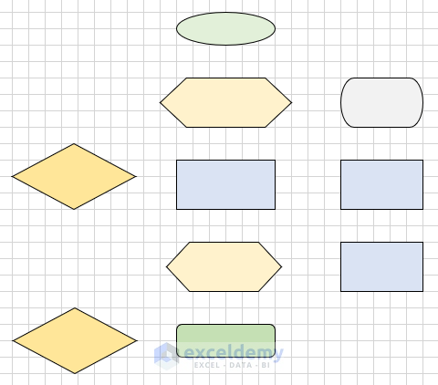
- Repeat the above steps to place all the shapes.
- Click any shape to get a Shape Format; you can edit the shapes.
- See the below figure where the input of the shapes is complete for this example.
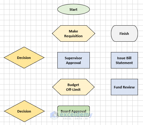
Method 5 – Add Text to Shapes
- Add texts, click the desired shape, and start typing.
- Format the texts if necessary by going to the Font, Alignment, etc. sections under the Home tab.
- The following image demonstrates the shapes along with the texts.
- The viewers can grasp the total concept more clearly by seeing the Flowchart.
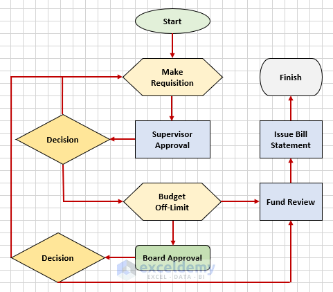
Method 6 – Connect Shapes to Make an Interactive Flowchart
- Join the shapes using Lines and Arrows. Arrows can distinctly show the directions of the workflow.
- Get those in the Shapes drop-down as we demonstrated in STEP 4. Look at the image below where our shapes are connected.
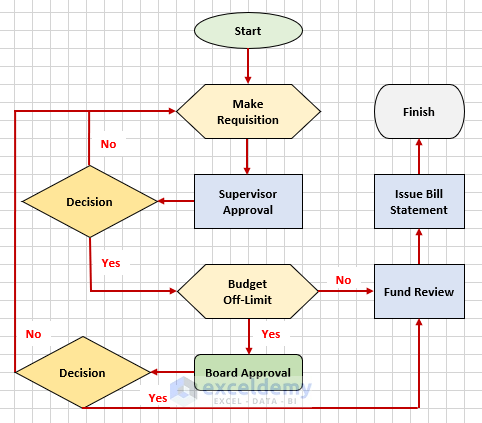
Method 7 – Attach Side Notes in Excel Flowchart
- Insert the notes using the Text Box, which you’ll find in the Shapes drop-down.
- The following image displays the Side Notes in the diagram.
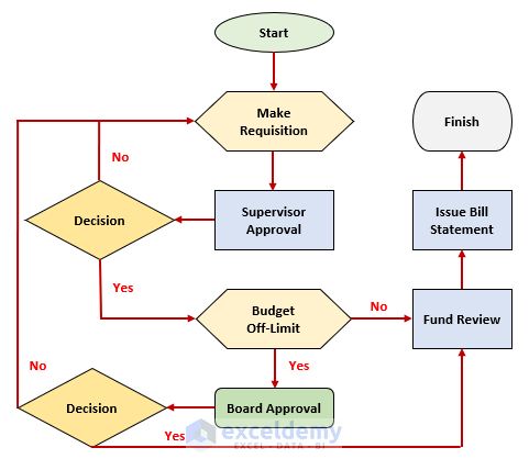
Final Output of an Interactive Flowchart
- Go to the Show section under the View tab to uncheck the Gridlines option.
- The Interactive Flowchart is designed.
- The following picture shows the final output of the Interactive Flowchart.
Download Practice Workbook
Download the following workbook to practice by yourself.
Related Article
<< Go Back to Flowchart in Excel | Learn Excel
Get FREE Advanced Excel Exercises with Solutions!
