How to Create a Chart from Selected Range of Cells in Excel

Get FREE Advanced Excel Exercises with Solutions!

Creating charts is one of the main purposes for which you use Excel. The different kinds of charts give us a visual representation of the data we are working on. In this article, I will show you how to create a chart from the selected range of cells in Excel in 4 efficient ways.


Create a Chart from Selected Range of Cells in Excel: 4 Efficient Ways

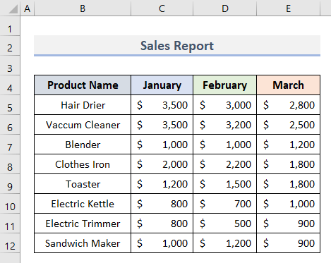
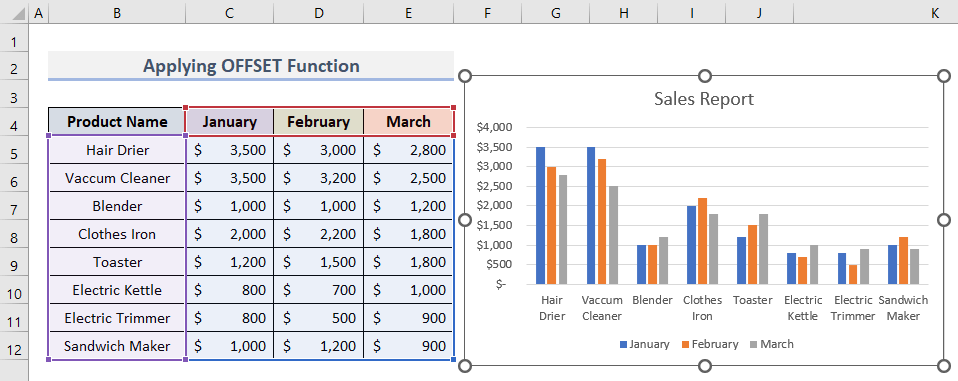
To describe the process, we have prepared a dataset. It shows the information of the Sales Report in the months of January, February, and March for 8 types of electric products.

How to Create a Chart from Selected Range of Cells in Excel


Now, we will create a chart out of this dataset. Let’s check the process below.

1. Create a Chart from Selected Cell Range Using an Excel Table

Normally while creating a chart you select the whole range of cells of your table. Before creating any chart, you create a table from which you can create different kinds of charts you want. In this process, making a graph or chart from a Table in Excel is very easy. Let’s see how it works.

  • In the beginning, go to the Home to and select Format as Table under the Styles group.

Create a Chart from Selected Cell Range Using an Excel Table

  • After making a table, select all the cells of your table while pressing the left button of your mouse.

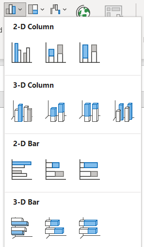
  • Following, press on to the Insert tab and select Bar Chart from the Charts section.

  • Then, select any chart you want.

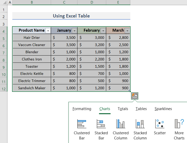
  • You can also insert the charts by selecting the range of cells and then clicking the right button of your mouse to select the Quick Analysis option.
  • After clicking the Quick Analysis option, you will see the Charts section.
  • Here, you can select any charts you want.

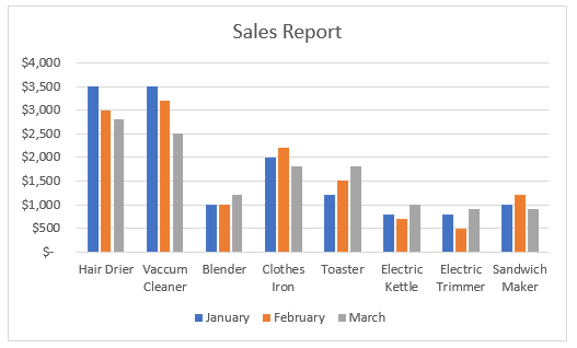
  • Finally, you will get to see the chart in your worksheet by applying any two of these methods.

Read More: How to Make an X-Y Graph in Excel


2. Apply OFFSET Function to Create Chart from Selected Cell Range

If you didn’t create a table but want to create a chart for various data, you can create Name Ranges and apply the OFFSET function further to run the process. For this follow the steps below:

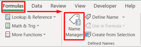
  • First, select the Formulas tab and then in the Defined Name section select the Name Manager.

Apply OFFSET Function to Create Chart from Selected Cell Range

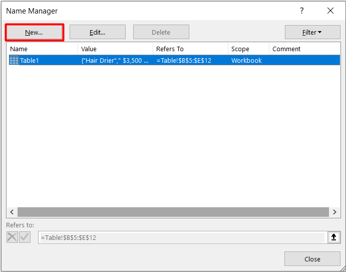
  • Afterward, you will find a new dialogue box.
  • Now, to create a new Name Range, select the New option.

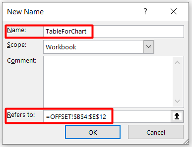
  • Following, in the New Name dialogue box, type TableForChart in the Name box.
  • Along with it, insert this formula in the Refers to box.
=OFFSET!$B$4:$E$12

Here, we applied the OFFSET function to facilitate modification after creating the chart. Because of this, whenever you insert or remove any data, the chart will automatically change accordingly.

  • After this, press OK.
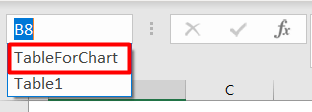
  • Now, you will find this Name Range in the Name Box.

  • After selecting the Name Range from the Name Box you will see that all the cells of this Name Range are selected.
  • Lastly, follow the same steps stated earlier to create any chart you want.

Note: Whenever the chart is created you will see the new chart name in the Name Box. So, don’t be confused if you see this.

Read More: How to Make a Graph in Excel That Updates Automatically


3. Modify Data Source to Create a Chart from Selected Range of Cells

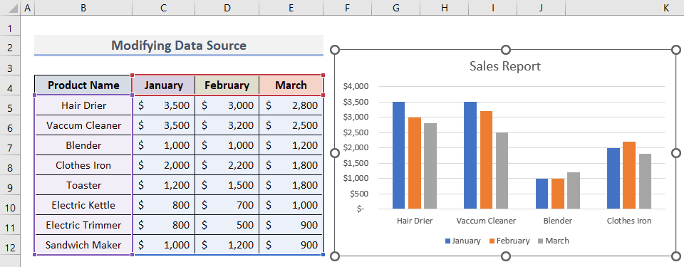
With the help of Name Range, you can even create new charts in an existing chart. Let’s see the process below:

  • First, select the existing chart.
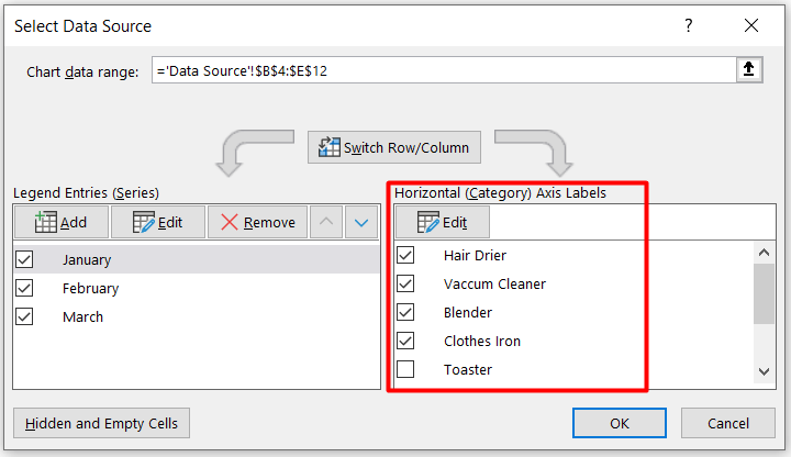
  • Then, click on the Design tab to select the Select Data option under the Data section.

Modify Data Source to Create a Chart from Selected Range of Cells

  • Now, in the Horizontal (Category) Axis Labels, select the categories you want in the chart.

  • Then, press OK.
  • Lastly, you will see a new chart in your worksheet which is different from the previous one.

Read More: How to Plot Graph in Excel with Multiple Y Axis


4. Select Specific Range of Cells for Creating a Chart in Excel

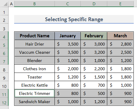
Suppose you don’t need some of the product information in your chart. The question arises what can you do? The answer is very simple. In this case, don’t select the information about those products which you don’t want to show in your chart. In my case, my table consists of 8 product names. I want to create a chat with 5 products. So, let’s follow the process below for this type of situation.

  • First, select all the relevant information for the 5 products in cell ranges B4:E7 and B11:E12. The information on the 3 products will not be selected.

Select Specific Range of Cells for Creating a Chart in Excel

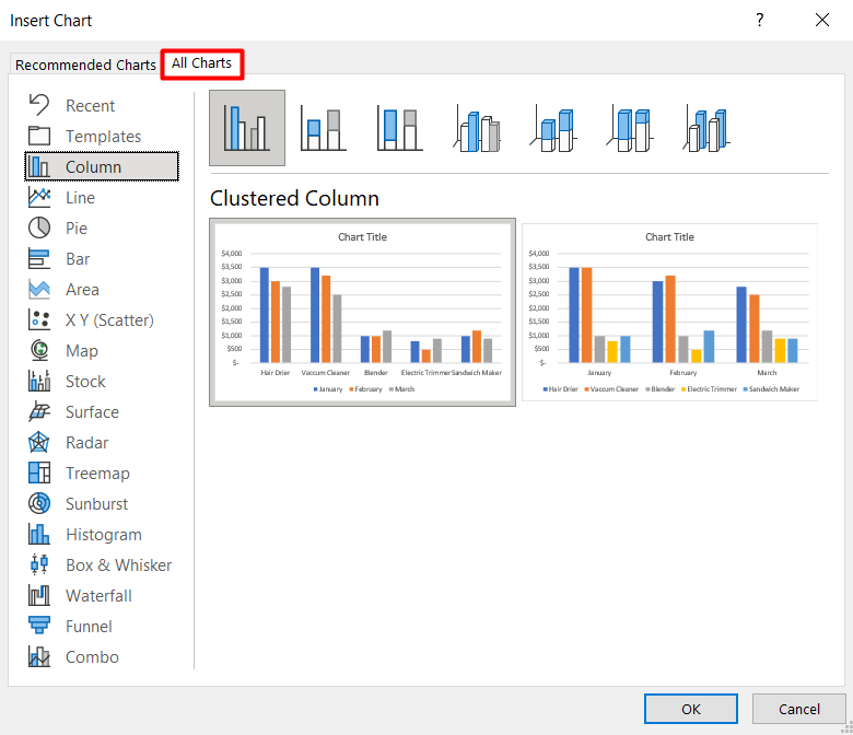
  • Next, go to the Insert tab and click on Recommended Charts.

  • Following, select any type of chart from the All Charts section.

  • Finally, press OK.
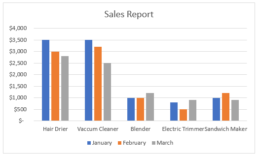
  • That’s it, you will see that only the selected product information will be shown in the chart.

Read More: How to Display Percentage in an Excel Graph


Things to Remember

  • Apply keyboard shortcut Ctrl + T for creating a table from your dataset.
  • When you add new data to the worksheet, it will automatically update the chart. Also, deleting any data will not entirely remove the data points from the chart.
  • Make sure there is no blank cell in the dataset.

Download Practice Workbook

Get this sample file and try the methods by yourself.


Conclusion

I hope after reading this article you will surely learn the process of how to create a chart from the selected range of cells in excel in 4 efficient ways. If you have any queries, place them in the comment box below.


<< Go Back To How to Create a Chart in Excel | Excel Charts | Learn Excel

What is ExcelDemy?

ExcelDemy - Learn Excel & Get Excel Solutions Center provides online Excel training , Excel consultancy services , free Excel tutorials, free support , and free Excel Templates for Excel professionals and businesses. Feel free to contact us with your Excel problems.
Siam Hasan Khan
Siam Hasan Khan

Hello! Welcome to my Profile. Here I will be posting articles related to Microsoft Excel. I have completed my BSc in Electrical and Electronic Engineering from American International University-Bangladesh. I am a diligent, goal-oriented engineer with an immense thirst for knowledge and an attitude to grow continuously. Continuous improvement and life-long learning are my mottoes.

1 Comment
  1. Very good, it help me a lot.

Leave a reply

Advanced Excel Exercises with Solutions PDF


ExcelDemy
Logo