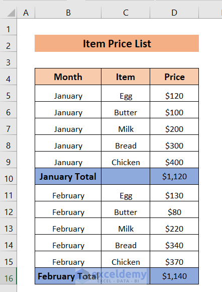
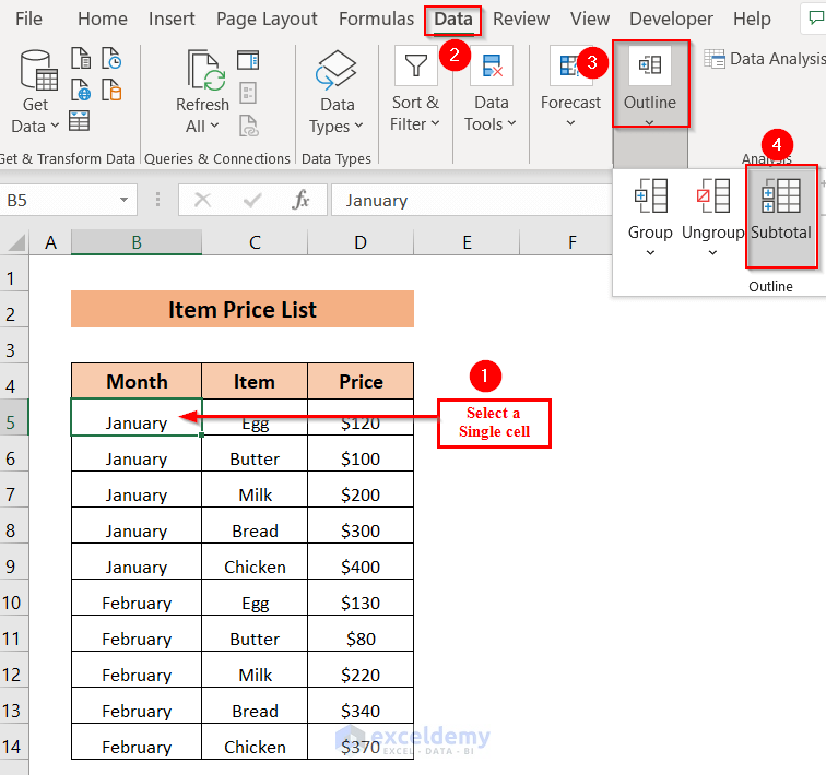
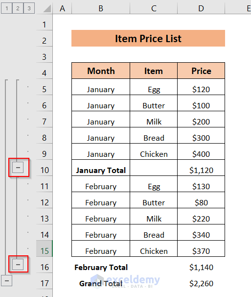
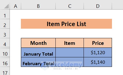
The following Item Price List table shows the Month, Item, and Price columns. We will collapse the rows of this table.
Method 1 – Creating Collapsible Rows in Excel Automatically
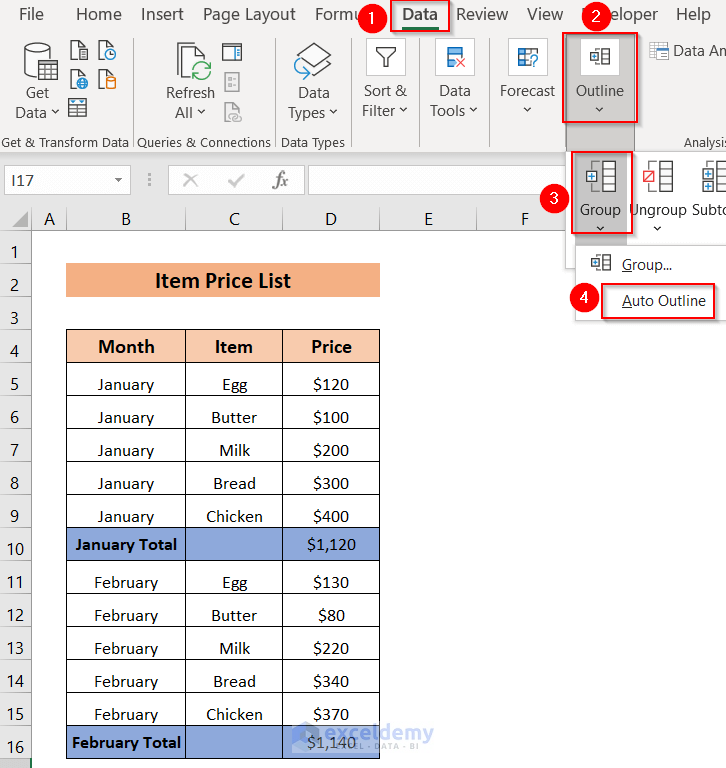
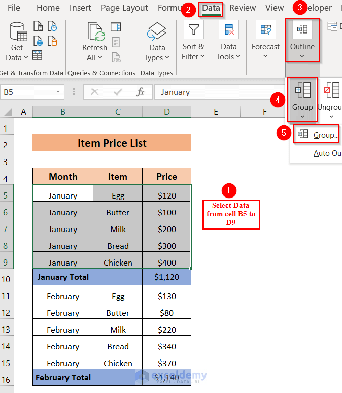
- Go to the Data tab in the ribbon.
- Select Outline, then choose Group and select Auto Outline.
- This creates two collapsible groups, with their numbers above the row headers to the left.
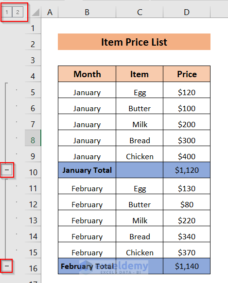
- Click on the minus sign on the row header to collapse the corresponding group (rows before it).
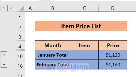
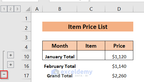
- We collapsed both groups, so we can only see the January Total and February Total rows. The other rows have been collapsed.
Read More: How to Expand or Collapse Rows with Plus Sign in Excel
Method 2 – Create Collapsible Rows Manually
We want collapsible rows for January, and we only want to see the January Total.
- Select the data from cells B5 to D9.
- Go to the Data tab, select Outline, then choose Group and pick Group…
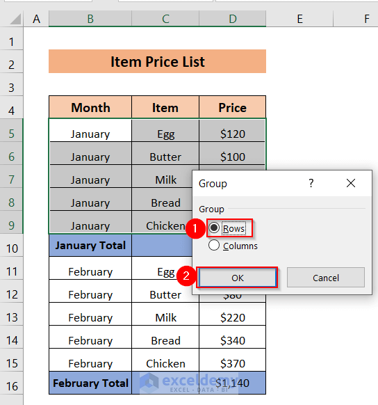
- A Group window will appear.
- Select Rows and click on OK.
- You’ll get a “–” sign on the left side of the January Total column, which indicates that the rows before that column will be collapsed.
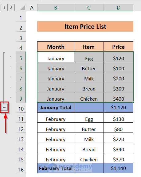
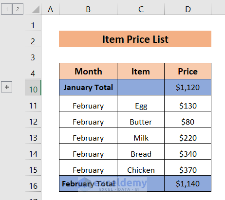
- If you click on the sign, all the rows before January Total have collapsed, and we only see January Total.
Read More: How to Expand and Collapse Rows in Excel
Method 3 – Using the Subtotal Option to Create Collapsible Rows in Excel
We want to calculate the total for January and February, and also we want to calculate the grand total for these two months.
- Select any cell of the table.
- Go to the Data tab and choose Outline, then select Subtotal.
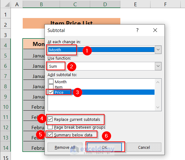
- A Subtotal window will appear.
- Select Month in the box At each change in.
- For Use function, pick Sum.
- For Add subtotal to, choose Price.
- Check Replace current subtotal and Summary below data.
- Hit OK.
- You’ll get three new rows named January Total, February Total, and Grand Total.
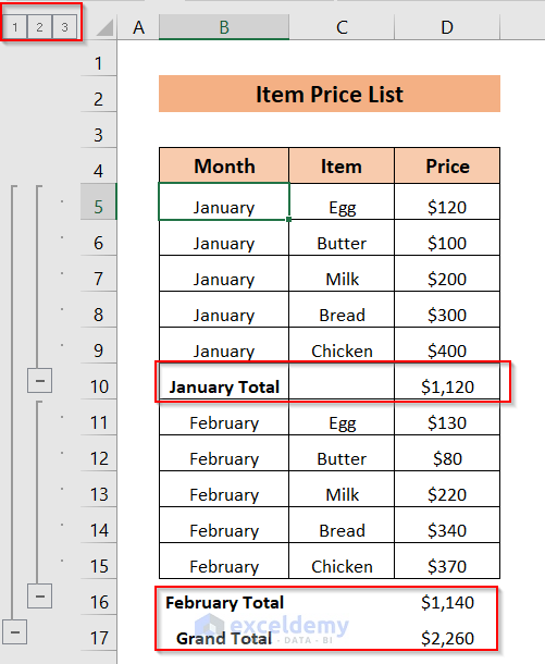
All rows have been created with the SUBTOTAL function.
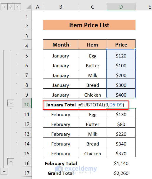
Let’s collapse the rows before the January Total and February Total rows.
- Click on the negative sign before the January Total and February Total rows.
- The rows before January Total and February Total have collapsed.
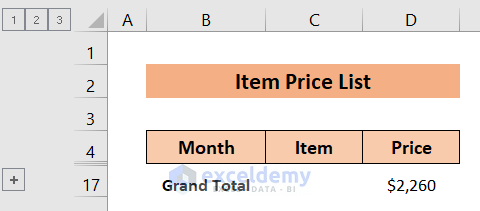
- You can also collapse the rows January Total and February Total and only see the Grand Total if you click on the negative sign before Grand Total.
- Here’s the result.
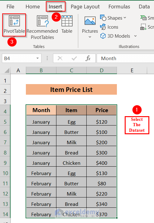
Method 4 – Creating Collapsible Rows with an Excel Pivot Table
- Select the entire dataset.
- Select Insert and choose PivotTable.
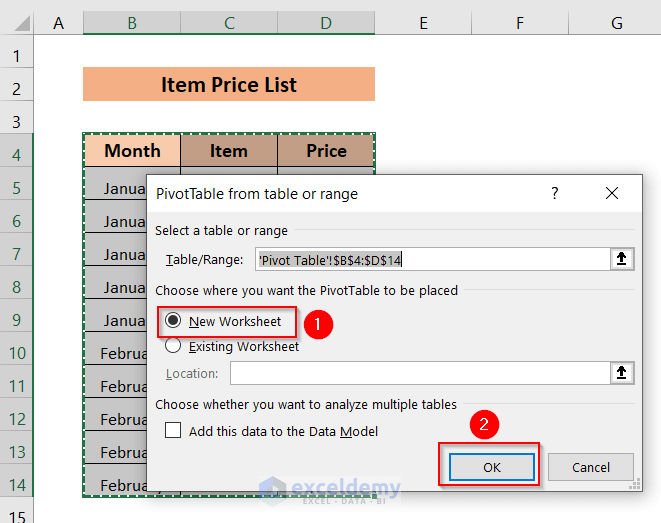
- A PivotTable from table or range window will appear.
- Select New Worksheet and click OK.
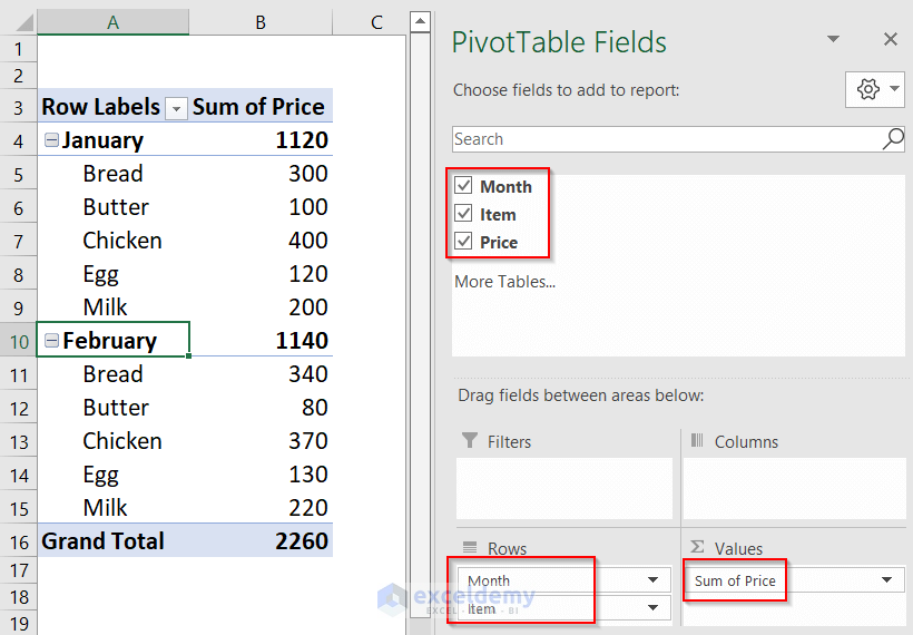
- Check Month, Item, and Price in PivotTable Fields.
- In the Rows, put Month and Item, and in the Values, put Sum of Price.
- Here’s the created Pivot Table.
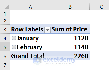
- To collapse the rows, click on the negative sign on the left side of January and February.
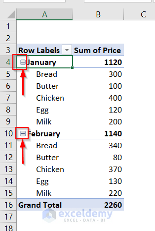
- We can see the rows with January, February and Grand Total. The rows in between have been collapsed.
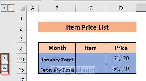
Hiding the Outline Symbols after Creating Collapsible Rows in Excel
We want to remove the plus sign before the January and February Total.
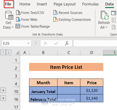
- Select the File tab in the ribbon.
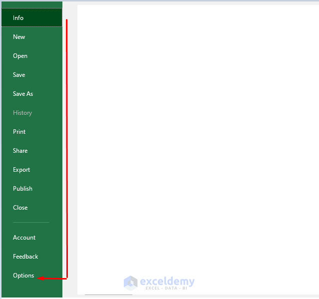
- Select Options.
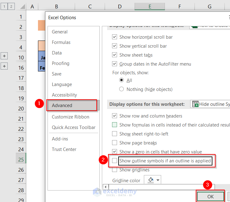
- Go to Advanced and unmark Show outline symbols if an outline is applied.
- Click OK.
- Here’s the result.
- You can check the option again to make the plus sign visible again
Download the Practice Workbook
Related Articles
- How to Lock Rows in Excel
- How to Color Alternate Rows in Excel
- How to Copy Every Nth Row in Excel
- How to Resize All Rows in Excel
- How to Create Rows within a Cell in Excel
<< Go Back to Rows in Excel | Learn Excel
Get FREE Advanced Excel Exercises with Solutions!
