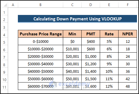
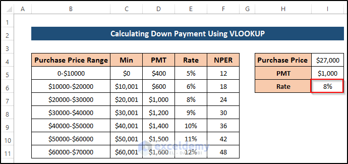
Step 1 – Create a Dataset
Create a purchase price range and enter the rate, the NPER, and the PMT.
Step 2 – Find the PMT Using the VLOOKUP Function
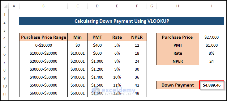
To find the PMT for a purchase price of $27000:
- Select I5.
- Enter the following formula.
=VLOOKUP(I4,$C$5:$D$11,2,TRUE)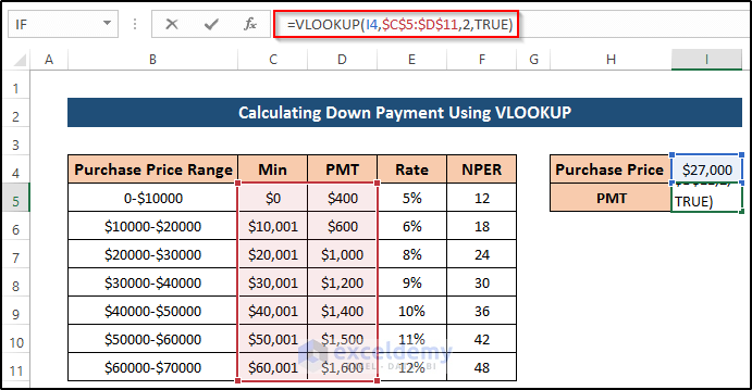
Formula Breakdown
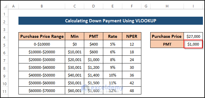
VLOOKUP(I4,$C$5:$D$11,2,TRUE): $27000 is the lookup value in I4. C5:D11 is assigned as table array The VLOOKUP function searches the lookup value in the table array. The column number to get the result is assigned. The PMT values are in the second column. True is set to an approximate match. For $27000, the VLOOKUP function returns $1000 PMT.
- Press Enter.
Read More: How to Calculate Auto Loan Payment in Excel
Step 3 – Calculate the Rate Using the VLOOKUP Function
- Select I6.
- Enter the following formula.
=VLOOKUP(I4,$C$5:$E$11,3,TRUE)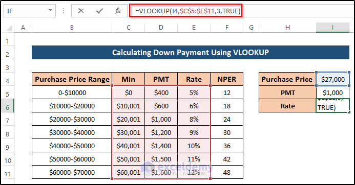
Formula Breakdown
VLOOKUP(I4,$C$5:$E$11,3,TRUE): $27000 is the lookup value in I4. E11. C5:E11 is assigned as table array The VLOOKUP function searches the lookup value in the table array. The column number to get the result is assigned. The Rate is in the third column. True is set to an approximate match. For $27000, the VLOOKUP function returns a Rate of 8%.
- Press Enter.
Step 4 – Calculate the NPER
- Select I7.
- Enter the following formula.
=VLOOKUP(I4,$C$5:$F$11,4,TRUE)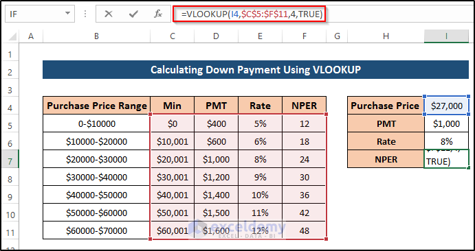
Formula Breakdown
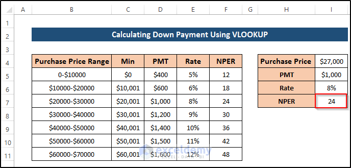
VLOOKUP(I4,$C$5:$F$11,4,TRUE): $27000 is the lookup value in cell I4. C5:F11 is assigned as table array The VLOOKUP function searches the lookup value in the table array. The column number to get the result is assigned.The NPER values are in the fourth column. True is set to an approximate match. For $27000, the VLOOKUP function returns the NPER value as 24.
- Press Enter.
Step 5: Calculate the Down Payment
- Select I10.
- Enter the following formula.
=I4-PV(I6/12,I7,-I5)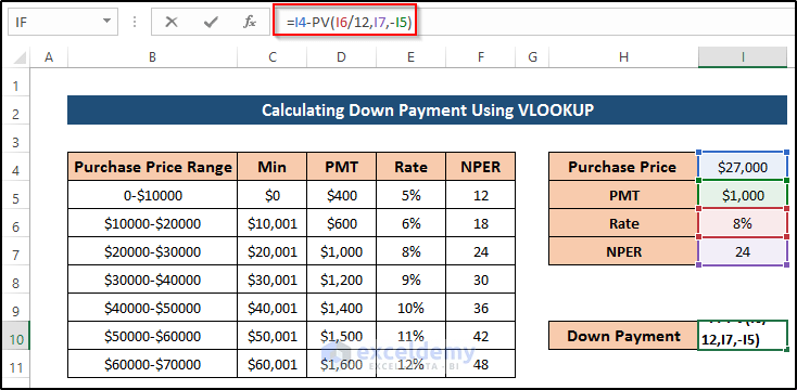
Formula Breakdown
I4-PV(I6/12,I7,-I5): The down payment amount is calculated by subtracting the value of the PV function from the purchase price. The PV function returns the loan amount or present value using Rate, NPER, and PMT. You need to calculate the monthly rate dividing it by 12 and subtracting it from the purchase price.
- Press Enter.
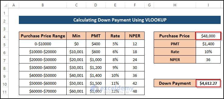
- If you change the purchase price from $27000 to $48000, the down payment will change.
Download Practice Workbook
Download the practice workbook.
Related Articles
- How to Calculate Monthly Payment with APR in Excel
- How to Calculate Balloon Payment in Excel
- How to Calculate Car Payment in Excel
- How to Calculate Coupon Payment in Excel
- How to Calculate a Lease Payment in Excel
<< Go Back to Calculate Payment in Excel | Excel for Finance | Learn Excel
Get FREE Advanced Excel Exercises with Solutions!
