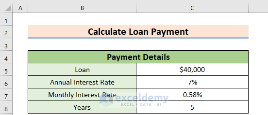
We will use the following dataset, which contains two columns with Payment Details.
Method 1 – Using the PMT Function to Calculate Loan Payments in Excel
Steps:
- Select a different cell C10, to keep the Monthly Payment.
- Use the following formula in the cell.
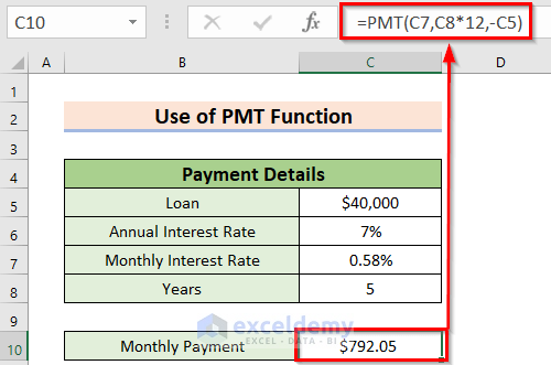
=PMT(C7,C8*12,-C5)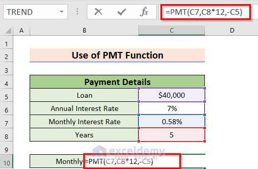
Formula Breakdown
We have used the PMT function which calculates the monthly or annual payment based on a loan with a constant interest rate and regular payment.
- C7 denotes the monthly interest rate of 0.58%.
- C8 denotes the total payment period in years which is 5. We have multiplied by 12 to calculate the monthly payment.
- C5 denotes the present value which is $40,000. The Minus sign denotes Loan as debit.
- Press Enter to get the Monthly Payment.
Read More: How to Calculate Auto Loan Payment in Excel
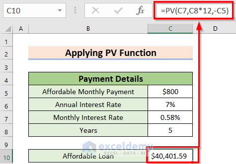
Method 2 – Use the PV Function to Calculate the Total Affordable Loan
We’ll use a potential Monthly Payment as given data.
Steps:
- Select cell C10, where you want to keep the Affordable Loan.
- Use the formula given below in the C10 cell.
=PV(C7,C8*12,-C5)- Press Enter to get the Affordable Loan.
Formula Breakdown
The PV function returns the present affordable amount of a Loan.
- C7 denotes the rate as the monthly interest rate.
- C8 denotes the total payment period in years which is 5. We multiplied by 12 for the monthly payments.
- C5 denotes the affordable monthly payment. The Minus sign denotes monthly payment as debit.
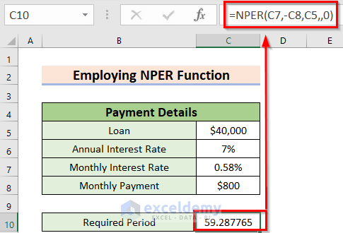
Method 3 – Using the NPER Function to Calculate the Required Payment Period
Steps:
- Select the C10 cell for calculating the required period.
- Use the following formula in the C10 cell.
=NPER(C7,-C8,C5,,0)- Press Enter to get the Required Period.
Formula Breakdown
The NPER function gives the required payment period in months.
- C7 denotes the monthly interest rate as Rate.
- C8 denotes payment made in each period as PMT. The Minus sign denotes monthly payment as debit.
- C5 denotes the total loan as present value (PV).
- As the Future Value is unknown, FV will be Blank.
- 0 denotes the type as ending of the period.
- Select cell C10.
- From the Home tab, go to the Number command.
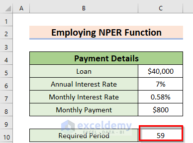
- Press the Decrease Decimal feature until the fractional number converts to a whole number.
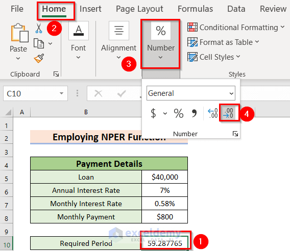
- The number is rounded down.
Read More: How to Calculate Monthly Mortgage Payment in Excel
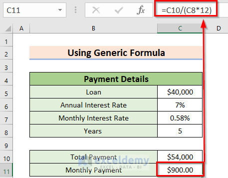
Method 4 – Use a Generic Formula to Calculate a Loan Payment in Excel
Steps:
- Select C10, where you want to keep the Total Payment.
- Use the formula given below in the C10 cell.
=C5*(1+C7*(C8*12))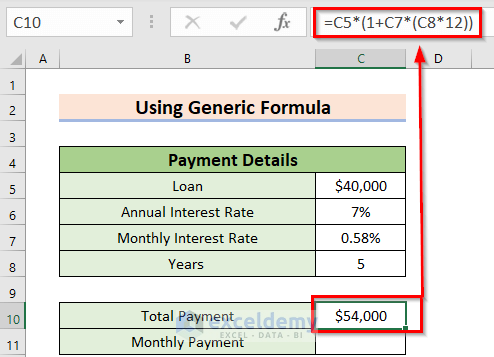
Formula Breakdown
- In this formula, we have converted years to months by multiplying 12 with C8 cell value.
- Output: 60.
- We multiplied the Monthly Interest Rate, C6 with 60.
- Output:0.35.
- We have added 1.
- Output: 1.35.
- We multiplied the whole result with the Loan, C5.
- Output: $54,000.
- Use the following formula in C11.
=C10/(C8*12)- Press Enter to get the result.
Read More: How to Calculate Monthly Payment with APR in Excel
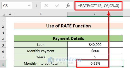
Calculating the Interest Rate of a Loan Payment in Excel
Steps:
- Select cell C8, where we’re keeping the Interest Rate.
- Use the following formula in the C8 cell.
=RATE(C7*12,-C6,C5,,0)- Press Enter to get the Interest Rate.
Formula Breakdown
The RATE function will return the monthly rate in percentage of Loan Payment.
- C7 denotes the NPER as the total payment period in years, which is 5. We have multiplied it by 12 for the monthly payment system.
- C6 denotes the payment made in each period as PMT. The Minus sign denotes the monthly payment as debit.
- C5 denotes the Loan as present value (PV).
- As the Future Value is unknown, FV will be Blank.
- 0 denotes the type as the ending of the period.
Things to Remember
- The four examples are for four different given information. Choose the method to do the calculation of Loan Payments according to your information.
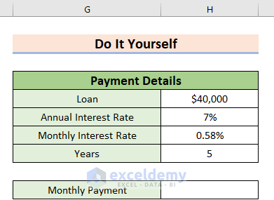
Practice Section
You can practice the explained methods on how to calculate loan payment in Excel by yourself.
Download the Practice Workbook
Related Articles
- How to Calculate Car Payment in Excel
- How to Calculate Coupon Payment in Excel
- How to Calculate a Lease Payment in Excel
- How to Calculate Down Payment in Excel Using VLOOKUP
- How to Calculate Balloon Payment in Excel
<< Go Back to Calculate Payment in Excel | Excel for Finance | Learn Excel
Get FREE Advanced Excel Exercises with Solutions!
