Latest Posts From Fahim Shahriyar Dipto

In the sample dataset below we have students' marks in the Theory and Practical courses. In this tutorial, we will add the marks to get the Total, and subtract ...

How to Plot a Graph in Excel You first need to plot a graph in Excel. Then you will be able to show the coordinates in that graph. It is possible that ...
Consider a dataset of student CGPAs with Student IDs. Some values are missing in Row 8 and Row 11. We'll remove rows with missing data from the ...

The image below showcases a chart of Month-wise Items Sold. The first 7 months of the year and items sold were used to create a chart. ...
Download the Practice Workbook Convert Time Zones.xlsx 3 Ways to Convert Time Zones in Excel Here is a dataset of individual times in London city ...

Suppose we have the dataset of students’ exam marks below. We want to know whose mark is between 40 and 60. In this article, we will use different formulas and ...

Method 1 - Compare Dates in Two Columns Whether They Are Equal or Not Steps: Select an appropriate cell (D5 in this example) and use the following ...

4 Major Reasons Why CTRL C Might Not Be Working in Excel Hardware problem can create the issue. The keyboard can malfunction so that CTRL C does not ...
Method 1 - Using Flash Fill Feature to Reverse Names in Excel Steps: Enter the first name in your desired order as shown below. Select the ...
- « Previous Page
- 1
- …
- 3
- 4
- 5
See Our Reviews at


Hello Ken K,
Thanks for your feedback. The Print Title options including Rows to Repeat are always disabled in the Print Preview’s page setup. Display the spreadsheet in Normal view, go to the Page Layout tab and click on Print Titles. You may check whether your worksheet is protected or not. If you are facing the same problem then your problem may be quite exceptional. So, we can not solve the problem without your Excel file. You can share your Excel file via [email protected].
Hopefully, we will be able to solve your problem. Keep supporting us.
Regards,
Fahim Shahriyar Dipto
Excel & VBA Content Developer.
To calculate the monthly lease payment in Excel, you can use the following formula:
=PMT(rate/12,nper,-PV,FV)where:
rate = the interest rate per period (in this case, 20% divided by 12 for monthly payments)
nper = the total number of periods (in this case, 36 months)
PV = the present value of the lease (in this case, the selling price plus maintenance and repair costs, or Rs 28440 + Rs 4500 = Rs 32940)
FV = the future value of the lease (in this case, the residual value, or 7.5% of the selling price, or Rs 2133)
In our dataset, in Cell C11 we entered the below formula.
=PMT(C9/12,C8,(-C6),C7,0)See the image for better visualization.
Hope you are able to calculate the monthly lease payment now. Have a nice day. Keep supporting us.
Regards,
Fahim Shahriyar Dipto
Excel and VBA Content Developer
Hello Pepe,
Thanks for your feedback. It’s a matter of upset that the Copy and Paste solution is not working in your Excel file. Whereas our method is working smoothly. You have to copy a chart and then paste it on another chart and your work will be done. As per your comment, the method doesn’t work. So, we have attached some steps to do that in an alternative way. Follow the below step.
1. Select the first chart, then right-click and choose “Copy“.
2. Click on the second chart to activate it.
3. Right-click on the chart area and choose “Paste” from the context menu.
4. You should now have two chart objects overlapping each other. You can resize and reposition them as desired.
5. Select the first chart, then right-click and choose “Format Chart Area” from the context menu.
6. In the Format Chart Area pane, under the Fill & Line tab, choose “No fill” and “No line“.
7. Repeat step 5 and 6 for the second chart.
Now you should have two charts merged into one.
If the above method fails then you can use the below method also.
1. Select the data range for both series.
2. Click on the “Insert” tab and choose “Recommended Charts“.
3. Scroll down to the “Combo” charts section and choose a chart type that suits your needs.
4. Click “OK” to create the chart.
5. Right-click on the chart and choose “Select Data” from the context menu.
6. In the “Select Data Source” dialog box, click the “Add” button to add a new series.
7. Select the data range for the second series and click “OK“.
You should now have a single chart with both series displayed.
Hope the above methods will work. If this doesn’t work then please send your excel file to [email protected]
Have a good day!
Regards
Fahim Shahriyar Dipto
Excel and VBA Content Developer.
Hello Anwer,
Thanks for your comment. It is the most common factor when you download a .xlsnm, the code doesn’t work. So, to avoid this consequence follow the steps stated below.
Firstly, download the .xlsm file from the article and right-click on the file. Select Properties.
Then, check the Unblock box and hit OK.
Hopefully, this method solves your issue. If not then change the directory of the file and Rename it at your preference. then the VBA code of the source file will run in the existing worksheet.
Again, if you are facing any obstacle then mail the Excel file to the address.
Regards,
Fahim Shahriyar Dipto
Excel & VBA Content Developer
Hello Terry,
It’s really nice to hear from you. In your query, you wanted to know about changing the plot area where the chart area will be the same. The VBA code needs to be modified a bit. I have attached the code below.
Sub Resize_Chart_Plot_Area()Dim ch1 As Chart, plot_height As Double, plot_width As DoubleSet ch1 = ActiveChartchart_height = ch1.PlotArea.Height: chart_width = ch1.PlotArea.Widthchart_height = ch1.PlotArea.Height: chart_width = ch1.PlotArea.Widthch1.PlotArea.Height = 150: ch1.PlotArea.Width = 400End SubRun the code with the F5 key and it will change the plot area without changing the plot area.
Have a great day.
Regards,
Fahim Shahriyar Dipto
Excel & VBA Content Developer.
Hello Jim,
Thanks for commenting. If I am not wrong, you want to sort dates that don’t have the dollar like the dataset below.
Select the entire data range then navigate the Home tab >> choose Sort & Filter from #diting group >> pick Filter.
Choose the Filter dropdown and uncheck the blanks from the column.
Finally, the dates are sorted with the dollar.
Regards
Fahim Shahriyar Dipto
Excel & VBA Content Developer
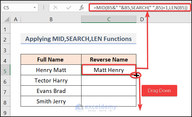
Hello Javate,
Thanks for commenting. Your query is similar to reverse names. You can do that in one column. For this, go to cell C5 and insert the following formula.
=MID(B5&","&B5,SEARCH(".",B5)+1,LEN(B5)+1)You have to use the MID, SEARCH, and LEN functions combinedly. You will get the output like the image below after pressing ENTER.
You can follow the Reverse Names in Excel article to get the proper idea also.
Hi Nathan,
Thanks for your valuable feedback. If I am not wrong, you want to count the characters without the symbols. For this factor, we have taken a sentence that contains commas. To remove the commas and count the characters insert the following formula in cell C5.
=LEN(SUBSTITUTE(B5," ",""))-LEN(B5)+LEN(SUBSTITUTE(B5,",",""))Press ENTER and get the following output.
It counts the total characters without commas.
Hi Quang,
Thanks for your feedback. You are right on this occasion. The formula will be
=(D15+E15)*F12in G16. unfortunately, we have made a mistake here. Thanks to you that you corrected us. We have updated the article.Best wishes to you.
Regards
Fahim Shahriyar Dipto
Excel & Content Developer.
Hi Anna,
Thanks for commenting. There are 13 commands under the Interior application. When you put a dot (.) after the Interior application you will find the commands. there are Color, Colorindex, Pattern, ThemeColor, etc in the command section. But all the commands have the built-in color code that’s why you won’t be able to choose a specific color using this code. but while you working with blanks you can insert the RGB command and the Custom Color Code. In our case, it is not possible as we have to maintain the same color for the duplicates. Hope, you understand our answer.
Regards,
Fahim Shahriyar Dipto
Excel & VBA Content Developer.
Hello Sumeet,
Thanks for commenting. You can download the Excel file and also the Pdf file of all the formulas Cheat Sheet. For your betterment, we attached the Excel file and Pdf File links here also.
Hello Espen,
First of all, thanks for commenting. it’s unfortunate that we don’t explain the line-shifting issues in this article. If I am not wrong, I think you are talking about the case like the image below.
For resolving the issue you can follow the procedure described in the method of Converting Word to Excel without splitting cells.You will get the result like the image below.
Hopefully, you will understand the steps mentioned in the link and solve your issue.
Have a nice day!
Regards
Fahim Shahriyar Dipto
Excel & VBA Content Developer
Hello Maurice,
Thanks for your feedback. In your query, as you wanted to create the combination for 3 columns and five rows, you have to change the VBA code variables to X1, X2, and X3. Also, you need to change the row range. Don’t worry, We have added the code for your betterment. Follow the code and your work will be done.
Sub CombinationsFor3Columns()Dim X1, X2, X3 As RangeDim RG As RangeDim xStr As StringDim FN1, FN2, FN3, FN4 As IntegerDim SV1, SV2, SV3, SV4 As StringSet X1 = Range("B5:B9")Set X2 = Range("C5:C9")Set X3 = Range("D5:D9")xStr = "-"Set RG = Range("D5")For FN1 = 1 To X1.CountSV1 = X1.Item(FN1).TextFor FN2 = 1 To X2.CountSV2 = X2.Item(FN2).TextFor FN3 = 1 To X3.CountSV3 = X3.Item(FN3).TextRG.Value = SV1 & xStr & SV2 & xStr & SV3Set RG = RG.Offset(1, 0)NextNextNextEnd SubHope the above code solves your problem. Keep supporting us.
Regards
Fahim Shahriyar Dipto
Excel & VBA Content Developer
Hello Fred,
Thanks for your appreciation. You can also do it for 4 columns also. All you need to change is the variable, integer and string. Without these changes, all the other code will be the same as before. We also provide the VBA code for the 4 columns below.
Sub CombinationsFor4Columns()Dim X1, X2, X3, X4 As RangeDim RG As RangeDim xStr As StringDim FN1, FN2, FN3, FN4 As IntegerDim SV1, SV2, SV3, SV4 As StringSet X1 = Range("B5:B7")Set X2 = Range("C5:C7")Set X3 = Range("D5:D7")Set X4 = Range("E5:E7")xStr = "-"Set RG = Range("H5")For FN1 = 1 To X1.CountSV1 = X1.Item(FN1).TextFor FN2 = 1 To X2.CountSV2 = X2.Item(FN2).TextFor FN3 = 1 To X3.CountSV3 = X3.Item(FN3).TextFor FN4 = 1 To X4.CountSV4 = X4.Item(FN4).TextRG.Value = SV1 & xStr & SV2 & xStr & SV3 & xStr & SV4Set RG = RG.Offset(1, 0)NextNextNextNextEnd SubHope the above code solves your problem. Keep supporting us.
Regards
Fahim Shahriyar Dipto
Excel & VBA Content Developer
Hello Euliin,
Thanks for commenting on our website. You can highlight a cell containing any random value with Conditional Formatting. Follow the steps.
Firstly, select the entire row that you want to be highlighted. Then go to the Conditional Formatting and choose New Rule.
Now, New Formatting Rule dialog box appears. Choose Use a formula which cells to format. Write the formula in the box in the Format values where this formula is true.
=OR(ISTEXT(B5),ISNUMBER(B5))And click on Format.
Now, Format Cells appears. Pick a color and hit OK.
Now, again hit OK in the New Formatting Rule box.
Finally, as you see you can highlight the row.
Hello Mr. Wilson,
Thanks for your valuable comment. If you want to paste only the value you can do it through Paste Special feature.
Firstly, create a dataset with the RANDBETWEEN function.
Whenever you press anything opening the file the numbers refresh automatically.
But, after copying the column with the CTRL + C key, right-click on the cell and choose Paste Special.
Paste Special dialog box appears. Check the Valuebox there and hit OK.
Finally, you have pasted the values without dragging anything.
I hope you got the solution. keep supporting us.
Regards,
Fahim Shahriyar Dipto
Excel & VBA content Developer.
Hello Siti,
First of all thanks for your feedback. You can follow the below article to solve your problem. Go through it and you will get the solution hopefully.
You can also use the following VBA code to merge multiple sheets into one and into separate sheets. But you have to put all the files into a specific folder and paste the folder path into the code. (mentioned in the article).
Sub ConsolidateFiles()Dim FileList, CurrentF As VariantDim nFiles, nSheets As IntegerDim cSh As WorksheetDim cWB, sWB As WorkbookFileList = Application.GetOpenFilename(FileFilter:="Microsoft Excel Workbooks (.xls;.xlsx;.xlsm),.xls;.xlsx;.xlsm", Title:="Choose Excel files to merge", MultiSelect:=True)If (vbBoolean <> VarType(FileList)) ThenIf (UBound(FileList) > 0) ThennFiles = 0nSheets = 0Application.ScreenUpdating = FalseApplication.Calculation = xlCalculationManualSet cWB = ActiveWorkbookFor Each CurrentF In FileListnFiles = nFiles + 1Set sWB = Workbooks.Open(Filename:=CurrentF)For Each cSh In sWB.SheetsnSheets = nSheets + 1cSh.Copy after:=cWB.Sheets(cWB.Sheets.Count)NextsWB.Close SaveChanges:=FalseNextApplication.ScreenUpdating = TrueApplication.Calculation = xlCalculationAutomaticEnd IfEnd IfEnd SubI hope you can get what you want after using the code. thanks again and keep supporting us.
Regards,
Fahim Shahriyar Dipto
Excel & VBA content Developer.
Hello Edho,
Thanks for your feedback. Though the question is quite unclear to us but we have tried another code for your working purpose.
Sub X()Set DataSet = Range("B4:D13")Interval = 3N = 4FormulaColumn = 3R = DataSet.Rows.CountIf R Mod Interval <> 0 ThenEnding = R + (Int(R / Interval) * N)ElseEnding = R + ((Int(R / Interval) - 1) * N)End IfFor i = (Interval + 1) To Ending Step IntervalFor j = 1 To NDataSet.Cells(i, FormulaColumn).EntireRow.InsertNext ji = i + NNext IFor i = 1 To EndingIf DataSet.Cells(i, FormulaColumn) = "" ThenDataSet.Cells(i - 1, FormulaColumn).CopyDataSet.Cells(i, FormulaColumn).PasteSpecial xlPasteFormulasEnd IfNext IApplication.CutCopyMode = FalseEnd SubLook at the code image carefully. We have changed the row number,N=4. It will insert 4 rows in after the active cell. We have put the FormulaColumn number 3 as our formula is existed in column 3. You can change the FormulaColumn number at your preference and the formula will be copied in your inserted rows for the exact formula column.
Hello Avery,
First of all, we would like to thank you for your appreciation. Again, thanks for taking the time to leave a comment about a problem that you’re facing. In our Excel file, the formula is working smoothly. You can follow the step-wise procedure thoroughly. If the problem in your file remains the same, then send the file to us. It will be easier for us to pinpoint the problem. We, the Exceldemy team, are always ready to solve users’ issues.
Regards,
Fahim Shahriyar Dipto
Excel and VBA Content Developer
Hello, Mrs. Thomas. Thanks for your feedback. You can easily show the day in the text by using the TEXT function. Follow the steps for better visualization.
Firstly, go to cell E5 and insert the method.
=TEXT(D5,"dddd")It will make the day in full form of the text.
Then press ENTER and drag it down for other cells with the Fill Handle tool.
Finally, you got your result.
For displaying the month in text go to the cell F5 and write up the formula.
=TEXT(D5,"mmmm")Drag down it and get the full result for the dates.
Hello Mr Martin. Thanks for your valuable feedback. We are grateful to you for informing us about the factor. According to your feedback, we cross-checked the issue. Unfortunately, the x and y values are switched unexpectedly somehow. we have updated the article. Thanks again.
Regards,
Fahim Shahriyar Dipto
Excel and VBA Content Developer.
Hello Nicol,
Here’s the solution. You can subtract two dates and can find out the days remaining in your hand. I have attached the step-by-step procedure for better understanding.
Firstly, go to cell E5 and insert the formula.
=C5-D5Secondly, press ENTER and drag down the Fill Handle tool.
Finally, you will get the result like the image below.
Hello Mr. Clark. Thanks for your valuable comment. In your query, you wanted to know about category-wise idea sorting. If I misunderstood your problem then please let me know about this. I am adding the sorted image here. Then I have described how I have done that.
Firstly, you need to set a list of ideas according to your category just like the image below.
Then in cell B5 write up the following formula.
=IF($B$4=J5,I5,"")Similarly, you have to put the same formula for the other columns but need to set the cell reference for the corresponding cells.
Then drag down the Fill handle Tool for C5, D5, E5 ad F5 cells to get the same formula.
Finally, you will get the result.
Now, if you want to add any category-wise idea then it will automatically be sorted in your dataset list. See the image for a better clarification.
First of all, Thanks Mr. Smith for your valuable feedback. its means a lot to us. For your query, we have attached the steps with the image. Hopefully, you will understand this.
To merge numerous Excel files into one, first, convert the XLSX files to CSV files. Navigate to the File Tab. Select the Save As option and then click the menu icon next to the Save Option. Then, in the list, you will find many file formats; explore them and select CSV UTF-8 (Comma delimited) from the list of other formats. Additionally, rename the file from Sales of January to 1-Sales of January (the serial numbers preceding the file name will arrange the files serially according to which serial we want to merge them). Finally, select the Save option.
Then we’ll have a new file with the new format, 1-Sales of January.csv.
To begin, Copy the path to the folder Multiple Files where we have saved our Excel files in CSV format to be combined.
When you press the WINDOWS key + R, the Run window will appear. To launch the command prompt, type cmd in the Open box and hit OK.
We’ve opened the CMD, or Command Prompt, as you can see.
Enter cd and a space after it. To paste the copied path of our Multiple Files folder, press CTRL+V or right-click on your mouse.
After clicking ENTER, you will be sent to the directory specified in the preceding line.
Now, in the new line, put copy *.csv Consolidate.csv (where Merged Worksheet is our new filename), followed by
After clicking ENTER, the following command lines will be created automatically, where we can see the two file names that we wish to combine.
After you close the CMD window, navigate to the Multiple Files folder, where you will find the new merged file titled Consolidate.csv.
When we view the Consolidate.csv file, we notice the Sales Record of January heading first, followed by the equivalent numbers from the February file.
Hopefully, we think the solution is helpful for you
Thanks for your appreciation. It means a lot. You can explore our website to find out extraordinary techniques in Excel.