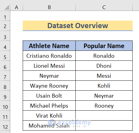
Here we have a dataset of a few famous athletes from different sports. Using this dataset, we will find partial matches within two columns.
How to Find Partial Match in Two Columns in Excel: 4 Easy Methods
Method 1 – Partial Match in Two Columns Using VLOOKUP
We will compare the two columns of the above dataset and produce the result in another column.
- Copy this formula into cell E5:
=IFERROR(VLOOKUP("*"&C5&"*";$B$5:$B$12;1;0);"")Here we have set the first row of the Popular Name column at the lookup_value field.
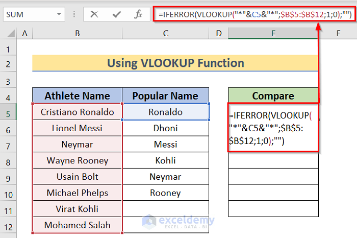
And the Athlete Name column as the lookup_array. Since we need to check partial match we have used the asterisk signs as wildcards. This sign denotes that any number of characters can be there.
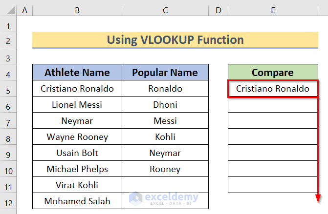
- When the match is found the formula will return the full name we selected in the cell.
- Use the Fill Handle option to apply the formula to all the cells.
- You will get the final result accordingly.
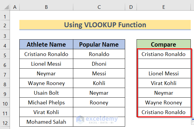
Note that, in cell E6, you have found a gap as the C6 cell contains the name Dhoni which the formula can’t find in Column B.
How Does the Formula Work?
Method 2 – Partial Match with Combination of INDEX – MATCH Functions
- Insert this formula into cell E5:
=IFERROR(INDEX($B$5:$B$12;MATCH("*"&C5&"*";$B$5:$B$12;0));"")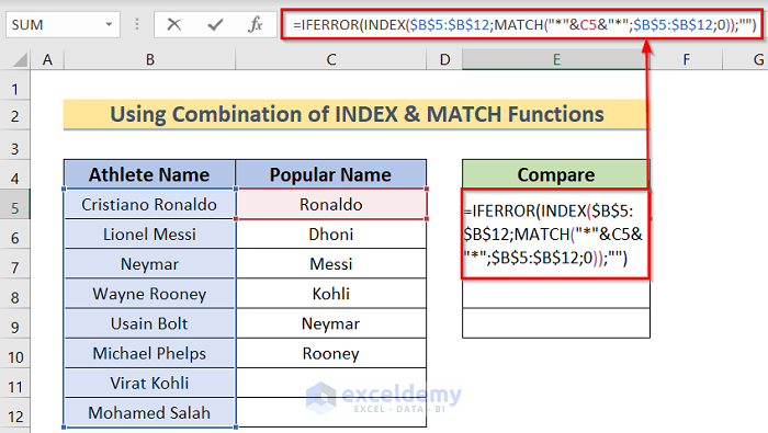
- Press Enter to get results for the cell and then use the Fill Handle to apply it to all cells.
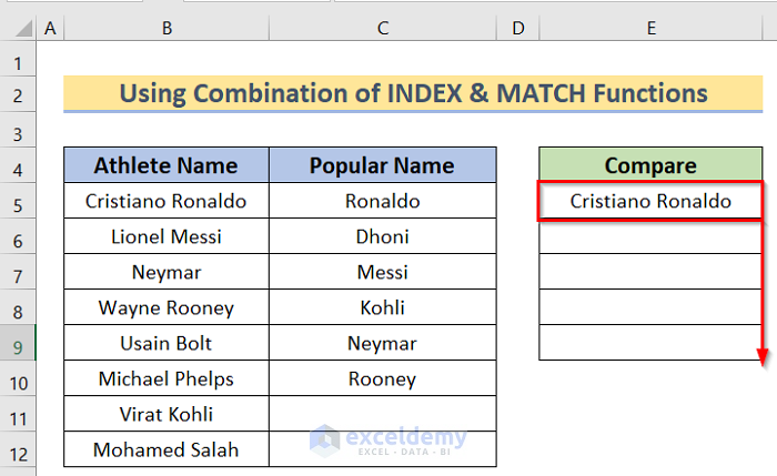
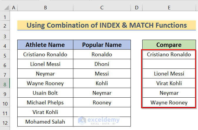
- You will get your final result.
- MATCH(“*”&C5&”*”;$B$5:$B$12;0): In the first portion, we will find the desired cell ranges we want to use.
- INDEX($B$5:$B$12; MATCH(“*”&C5&”*”;$B$5:$B$12;0)): When you intend to return a value (or values) from a single range, you will use the array form of the INDEX function. This portion will apply the proper criteria in the formula.
- IFERROR(INDEX($B$5:$B$12; MATCH(“*”&C5&”*”;$B$5:$B$12;0));””): This will take the ranges from the INDEX and MATCH function portion and set the proper condition for the formula.
The IFERROR function ignores any kind of error that may occur because of any inconsistency in the formula.
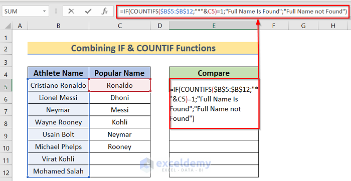
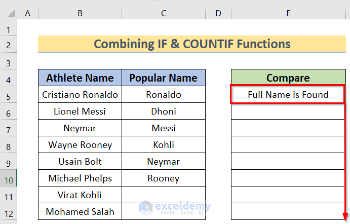
Method 3 – IF Function to Perform Partial Match in Two Columns
- Use the following formula for E5:
=IF(COUNTIFS($B$5:$B$12;"*"&C5)=1;"Full Name Is Found";"Full Name not Found")We have set the “Full name Is Found” as the if_true_value and left the if_false_value empty.
Here the formula provided the if_true_value.
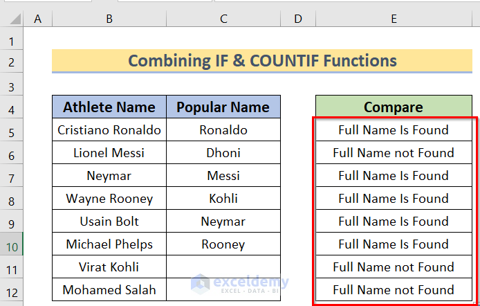
- After pressing the Enter button, use the Fill Handle option to copy the formula across the column.
- You will get the desired result.
How Does the Formula Work?
- COUNTIFS($B$5:$B$12;”*”&C5): In the first portion, we will find the range of the cells that we want to check with the condition.
- IF(COUNTIFS($B$5:$B$12;”*”&C5)=1; “Full Name Is Found”; “Full Name not Found”): This portion will apply the proper criteria in the formula.
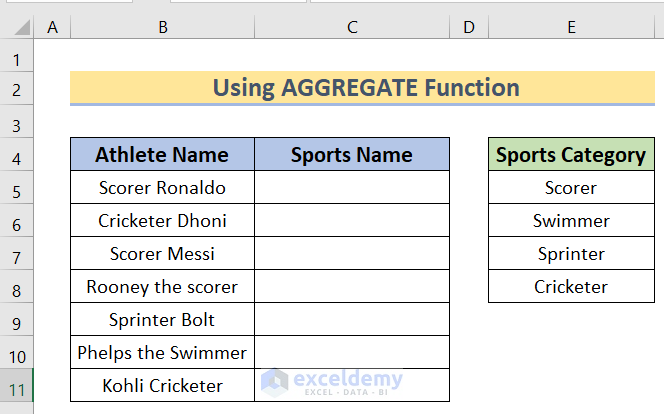
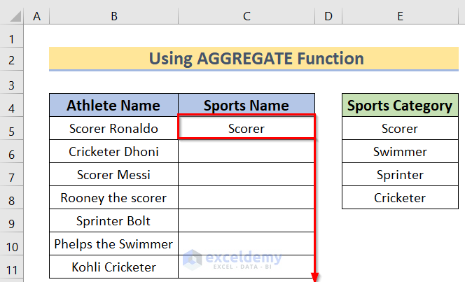
Method 4 – Compare Two Columns Using AGGREGATE Function
Microsoft Excel functions like SUM, COUNT, LARGE and MAX won’t function if a range contains errors. However, you can quickly solve this by using the AGGREGATE function.
AGGREGATE Function: Syntax and Arguments
Excel’s AGGREGATE function returns the aggregate of a data table or data list. A function number serves as the first argument, while various data sets make up the other arguments. To know which function to employ, one needs to memorize the function number, or beside you can see it in the table.
Reference and array syntax are the two possible syntaxes for the Excel AGGREGATE function which we will show you here.
Array Syntax:
=AGGREGATE(function_num,options,array,[k])
Reference Syntax:
=AGGREGATE(function_num,options,ref1, [ref2],…)
Based on the input parameters you supply, Excel will choose the most suitable form.
Arguments:
| Function | Function_number |
|---|---|
| AVERAGE | 1 |
| COUNT | 2 |
| CONTACT | 3 |
| MAX | 4 |
| MIN | 5 |
| PRODUCT | 6 |
| SUM | 9 |
| LARGE | 14 |
| SMALL | 15 |
Steps:
- Insert the following formula in the cell:
=@INDEX(E$5:E$8;AGGREGATE(15;6;MATCH("*"&$E$5:$E$8&"*";$B5;0)*(ROW($E$5:$E$8)-ROW(E$5)+1);1))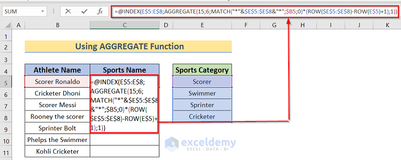
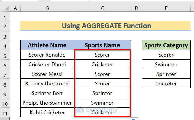
- You will get the result for this cell. Use the Fill Handle option to apply it to all cells.
- Your screen will show a result similar to the following image.
How Does the Formula Work?
Download Practice Workbook
You can download the practice workbook from here.
<< Go Back to Partial Match Excel | Formula List | Learn Excel
Get FREE Advanced Excel Exercises with Solutions!
