We often need to use the same table in multiple sheets for calculation and analysis. Copying the entire table and pasting it wherever we need is a very efficient way for small tables, but for large tables it’s impractical. Mirroring the table is an effective solution.
Mirroring means making a copy of the table where changes in the main table reflect in the secondary or copied table in real-time.
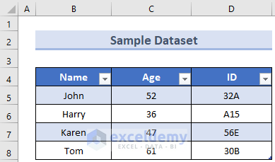
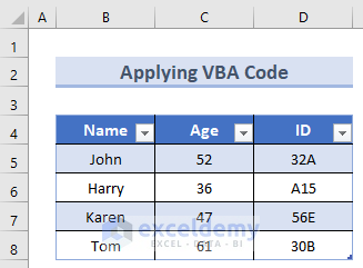
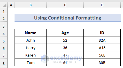
To illustrate our methods for creating table mirrors, we will use the following table:
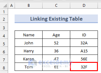
Method 1 – Linking an Existing Table on Another Sheet
If we create a table on the second sheet that is totally dependent on the main table, every time we update the main table, the dependent table will automatically update itself.
Steps:
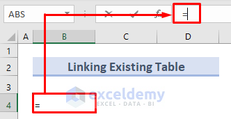
- Select the cell on the second sheet where we want to start our table. Here, cell D4.
- While the cell is selected, type‘=’ in the formula bar and click on the sheet tab that contains the main table.
- Select the entire main table.
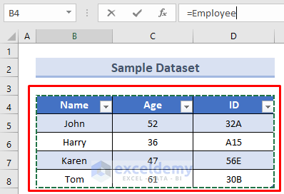
- Press Enter.
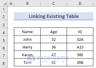
The entire table is copied, and any changes made to the main table will reflect in this table as well.
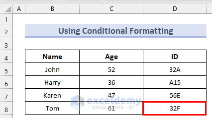
To illustrate, let’s change the data in the first table. For example, we changed Tom’s ID to 32F.
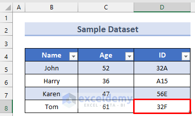
The mirrored table changes accordingly.
Read More: How to Create Table from Another Table in Excel
Method 2 – Using Microsoft Query
This method is also appropriate for mirroring a table in different workbooks.
Steps:
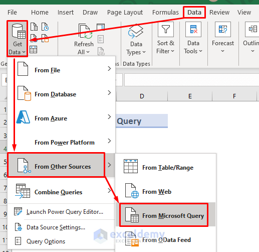
- Go to the Data tab in Ribbon.
- Click Get Data > From Other Sources > From Microsoft Query.
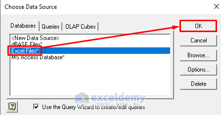
A Choose Data Source dialog box will appear.
- Click on Excel Files*.
- Click OK.
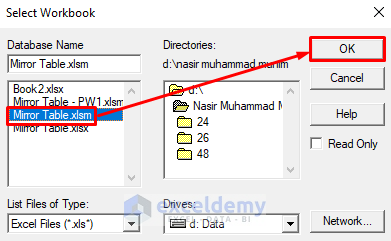
A file selection box will appear.
- Locate the file location of the file we are working on. If it’s not saved, save it first and try again.
- After selecting the file, click OK.
The Query Wizard will appear.
- Select the table you want to mirror and click on the ‘>’ button.
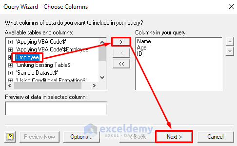
All the columns of that table will be displayed.
- Click on the Next button in the next 2 dialog boxes and select Finish in the last one.
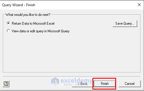
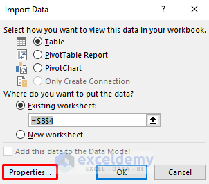
A small dialog box will appear asking for the location where you want to store the table.
- Select the destination cell.
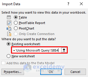
- Click on Properties.
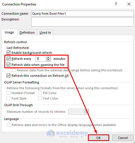
A new dialog box named Connection Properties will appear.
- Tick Refresh every and Refresh data when opening the file.
- In the Refresh every option, input your desired interval for how frequently you want to update the table with any changes.
- Click OK in both dialog boxes to complete the process.
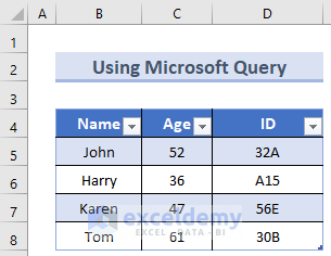
A mirrored table appears, where data will be updated according to the time interval we just set.
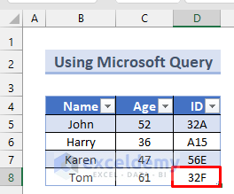
To illustrate, let’s change some data in the first table. For example, we changed Tom’s ID to 32F.

As we set Refresh to every 1 minute, the change will appear in the mirrored table after 1 minute.
Read More: How to Create Table from Another Table with Criteria in Excel
Method 3 – Applying VBA
When working with a large function or work process, using the VBA method will avoid complexity and save operational time.
Steps:
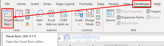
- Go to the Developer tab in the Ribbon.
- Select Visual Basic.
- Alternatively, press Alt+F11.
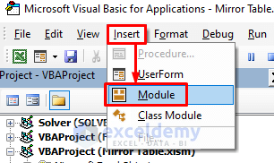
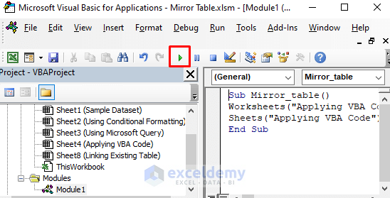
A window will appear named Microsoft Visual Basic for Application.
- Click on Insert and select Module.
- In that Module, enter the following code:
Sub Mirror_table()

Worksheets("Applying VBA Code").Range("B4:D8").Value = _
Worksheets("Sample Dataset").Range("B4:D8").Value

Sheets("Applying VBA Code").ListObjects.Add(xlSrcRange, _
Range("B4:D8"), , xlYes).Name = "Tablev"

End Sub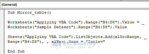
Code Breakdown
- Here we created a Subroutine to mirror a table.
- We used the Range.Value to get the values of the original table.
- We used Sheets().ListObjects.Add().Name to convert the values into a new table.
- Double-click on the sheet to apply the VBA subroutine. In our case, the sheet is Sheet4.
- Copy and paste the following code into the box that appears:
Private Sub Worksheet_Activate()
Call Mirror_table
ThisWorkbook.RefreshAll
End Sub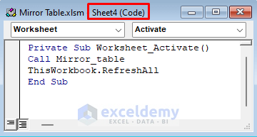
Code Breakdown
- To create a Private Sub, we selected Worksheet from General and selected Activate as an event from declarations. Now, whenever we activate the sheet, the code will run automatically.
- We then used a Call Statement to call the Sub procedure named Mirror_Table.
- Finally, we used the VBA Refresh.All property within Thisworkbook so that whenever the sheet is activated, the entire workbook will be refreshed.
- Press the Run icon in that window.
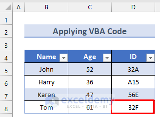
The following table will be created, which will update automatically every time the main sheet or Sample Dataset is updated.
Let’s modify the main dataset to test our code as before.

Open Sheet4 again, and the changes will have been applied.
Read More: How to Create Table from Multiple Sheets in Excel
Method 4 – Using a Conditional Formula
We can also use the IF function and conditions to create a mirrored table.
Steps:
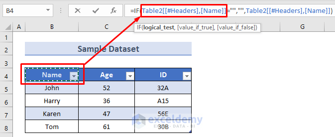
- Select the cell where we will start our table. In our case, cell B4.
- Enter this formula in the formula bar:
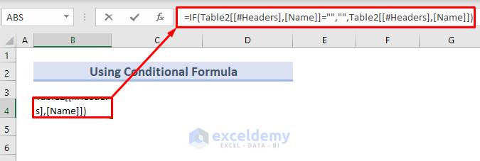
Here Table2[[#Headers],[Name]] can be replaced as required as follows:
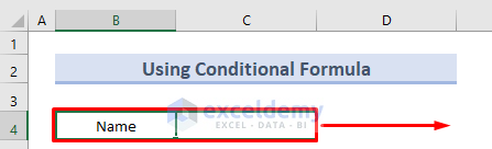
- Select the cell.
- Enter ‘=’ in it
- Go to the worksheet containing the main table.
- Select the top left table heading.
- Press Enter.
- The top left table header will appear in cell B4.
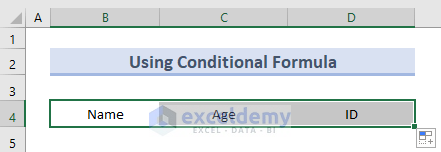
- Drag the Fill Handle right, horizontally, to mirror all the table headers.
All the table headers will be mirrored.
- Drag the Fill Handle down to automatically fill the rest of the data.
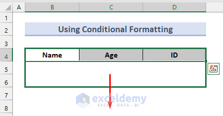
The end result will look like this:
If we now modify some data as in the previous Methods, the changes will reflect automatically.
Read More: How to Create a Lookup Table in Excel
Things to Remember
- Linking Existing Table and Using Conditional Formula methods will only return the values of those cells. So, the output is not strictly a table. To get the table form, we will need to format it as a table again.
- In the VBA method, the second code refreshes the worksheet, which is necessary to update changes made to the main table.
- The query can be refreshed manually by going to the Data tab and pressing the Refresh All option.
Download Practice Workbook
Related Articles
- How to Make 3D Table in Excel
- How to Make a Conversion Table in Excel
- How to Make a Decision Table in Excel
- How to Create a League Table in Excel
- How to Make a Table Bigger in Excel
<< Go Back to Make a Table | Excel Table | Learn Excel
Get FREE Advanced Excel Exercises with Solutions!

When you add a line or column to the source table this is not duplicated in the duplicate table. Is it possible to duplicate a table including when you add or remove lines or columns?
Hello Jude Ranby,
Here, the first methods Linking Existing Table on Another Sheet in Excel is duplicating the source table.
Here, I’m attaching a video for understanding.
Regards
ExcelDemy