If you are looking for ways to calculate GPA in Excel, then this article will serve this purpose. GPA is the acronym for Grade Point Average. The GPA of a student influences the chances of getting scholarships and grants for their future studies. For this reason, students need to keep track of their GPA. By using Excel, you can easily calculate your own GPA by following some simple steps. So let’s start with the article and learn all these steps to calculate GPA in Excel.
3 Simple Steps to Calculate GPA in Excel
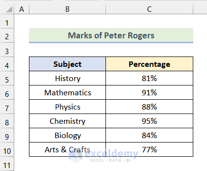
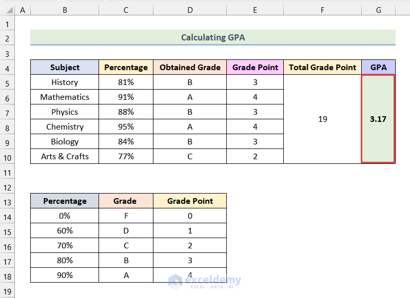
In this article section, we will learn about the 3 simple steps to calculate GPA in Excel. In the following dataset, we have the Marks of 6 Subjects of Peter Rogers, a 9th Grade student. Our aim is to calculate GPA of Peter Rogers.
We have used Microsoft Excel 365 version for this article, you can use any other version according to your convenience.
Step-01: Creating Reference Table to Calculate GPA
Firstly, we need to create a Reference Table where the Percentage ranges of different Grades along with the Grade Points are provided. Let’s follow the steps mentioned below.
- Firstly, create a table with 3 columns and 6 rows.
- After that, name the columns as Percentage, Grade, and Grade Point respectively.
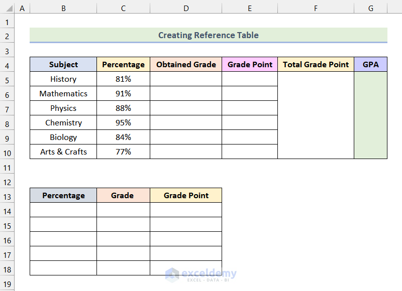
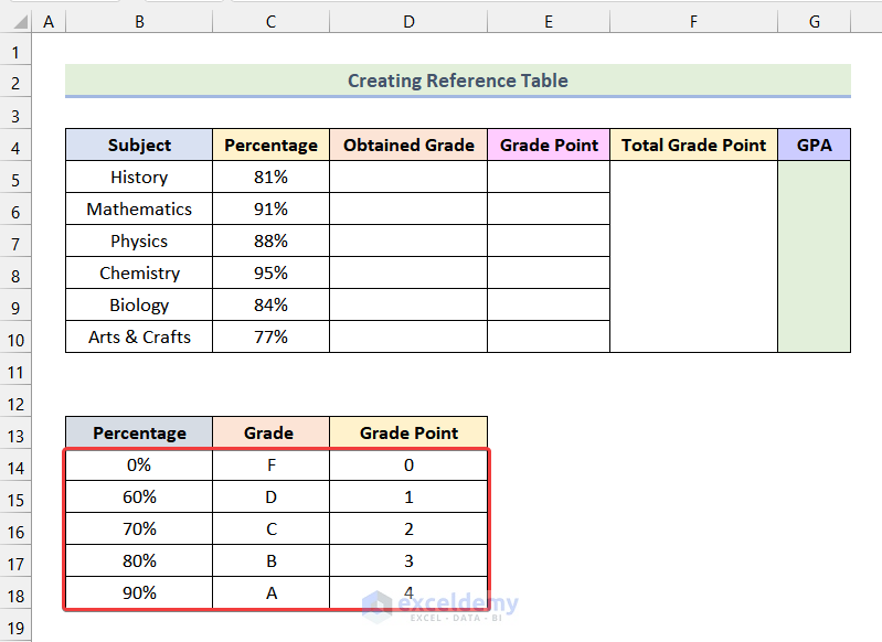
- Now, enter the Percentage ranges, Grades, and Grade Points as shown in the following picture.
Read More: How to Calculate College GPA in Excel
Step-02: Using VLOOKUP Function to Calculate GPA in Excel
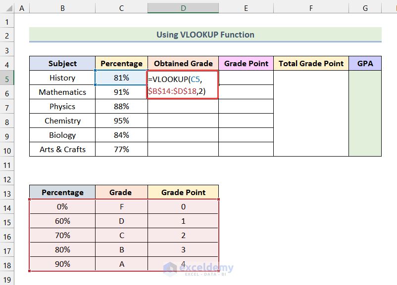
In this step, we will use the VLOOKUP function to determine the Obtained Grade and the Grade Point of each Subject. To do this, we will use the procedure discussed below.
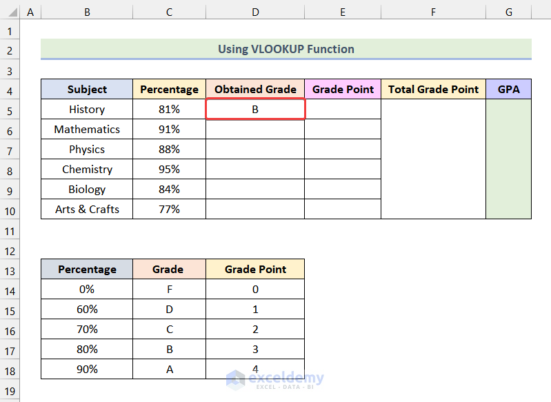
- Firstly, enter the following formula in cell D5.
=VLOOKUP(C5,$B$14:$D$18,2)Here, cell C5 refers to the obtained Percentage of History exam, the range $B$14:$D$18 represents the Reference Table that we are using to calculate GPA.
Formula Breakdown
- =VLOOKUP(C5,$B$14:$D$18,2) → It looks for a given value in the leftmost column of a given table and then returns a value in the same row from a specified column.
- C5 → lookup_value argument.
- $B$14:$D$18 → table_array argument
- 2 → col_index_num argument
- Output → B
- Following that, press ENTER.
Consequently, you will see the Grade of History as marked in the image given below.
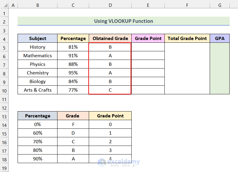
- Next, use the AutoFill feature of Excel to get the rest of the Grades for other Subjects as shown in the following picture.
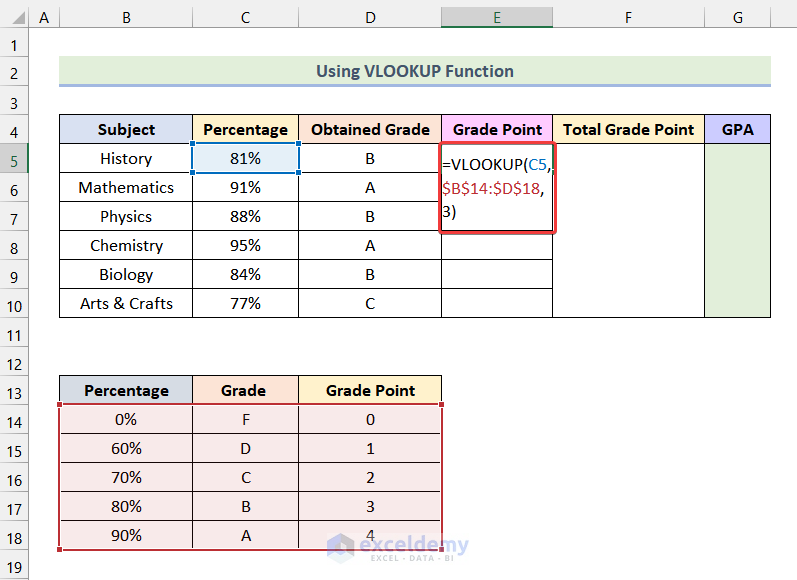
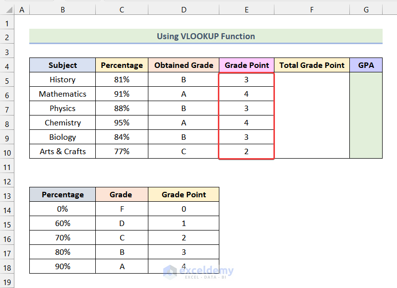
- Now, enter the formula given below in cell E5.
=VLOOKUP(C5,$B$14:$D$18,3)Formula Breakdown
- =VLOOKUP(C5,$B$14:$D$18,2) → It looks for a given value in the leftmost column of a given table and then returns a value in the same row from a specified column.
- C5 → lookup_value argument.
- $B$14:$D$18 → table_array argument
- 3 → col_index_num argument
- Output → 3
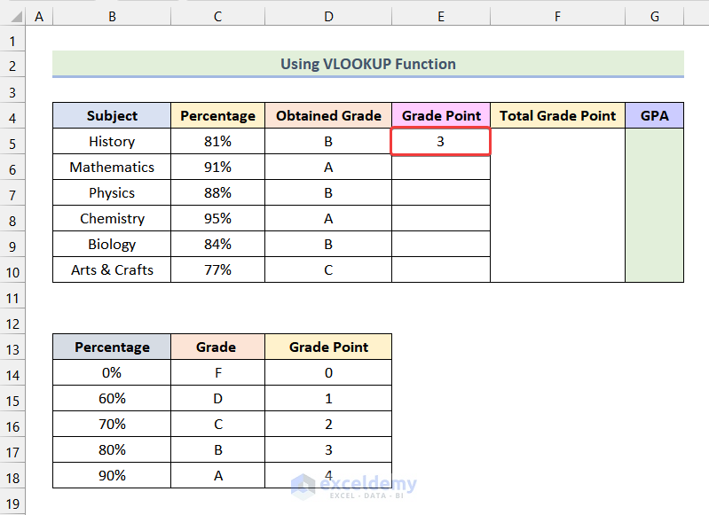
- After that, hit ENTER.
As a result, the Grade Point of History for Peter Rogers will be available in cell E5 as marked in the below-given picture.
- Afterward, by using the AutoFill option of Excel, you can obtain the remaining Grade Points for the rest of the Subjects.
Read More: How to Make a Grade Calculator in Excel
Step-03: Utilizing SUM and COUNTA Functions to Calculate GPA
First, we will use the SUM function to calculate the Total Grade Point. To do this, let’s follow the steps given below.
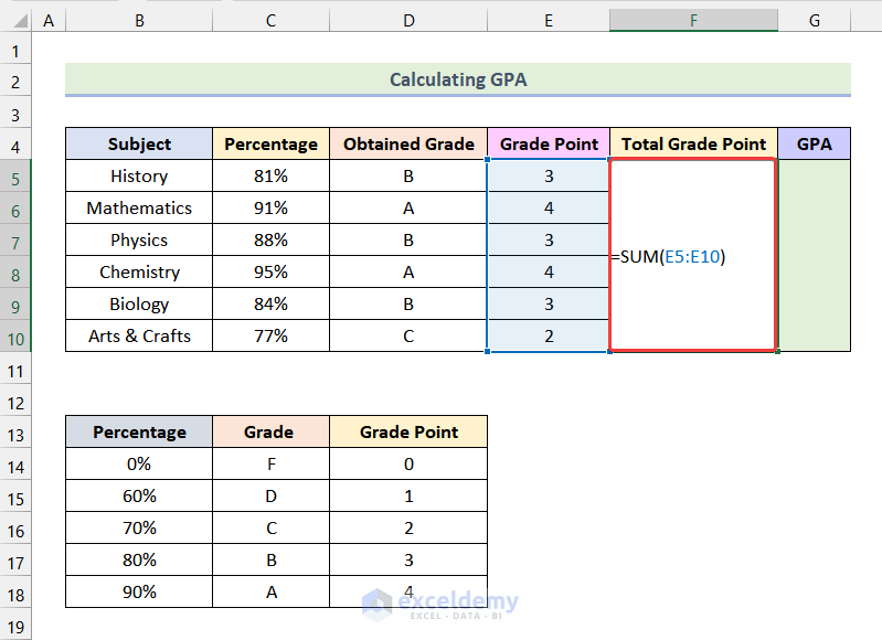
- Firstly, enter the following formula in cell F5.
=SUM(E5:E10)Here, the range E5:E10 represents the Grade Points achieved by Peter Rogers in different Subjects.
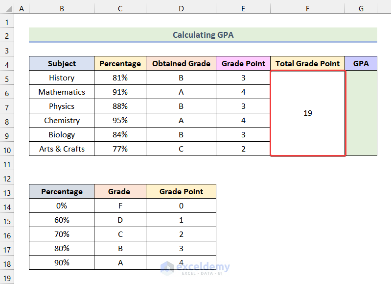
- Following that, press ENTER.
Subsequently, you will see the Total Grade Point in cell F5 as marked in the following picture.
Finally, to calculate the GPA, we will use the COUNTA function. Now, follow the steps that are discussed below.
- Firstly, enter the formula given below in cell G5.
=F5/COUNTA(B5:B10)Here, the range B5:B10 refers to the cells of the column Subject.
- Then, hit ENTER.
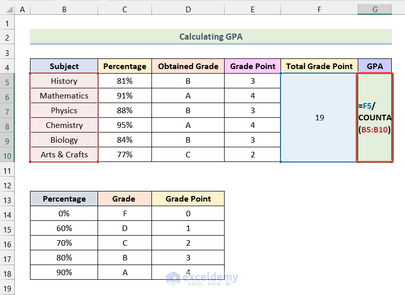
Consequently, you will see the GPA obtained by Peter Rogers in cell G5 as demonstrated in the following picture.
Read More: How to Calculate Grades with Weighted Percentages in Excel
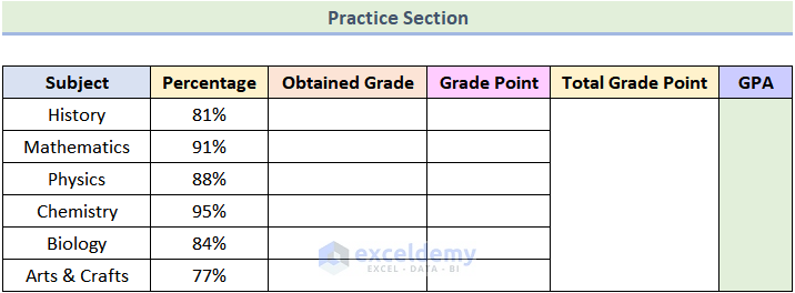
Practice Section
In the Excel Workbook, we have provided a Practice Section on the right side of the final worksheet. Please practice it by yourself.
Download Practice Workbook
Conclusion
Finally, we have to the end of the article. I sincerely hope this article could guide you in calculating GPA in Excel. Please feel free to leave a comment if you have any queries or recommendations for improving the article’s quality.
Related Articles
- How to Calculate Average Percentage Increase for Marks in Excel Formula
- How to Average Letter Grades in Excel
- Make Result Sheet in Excel
- How to Make Automatic Marksheet in Excel
- How to Calculate Subject Wise Pass or Fail with Formula in Excel
- How to Calculate Final Grade in Excel
- How to Calculate Average Percentage of Marks in Excel

