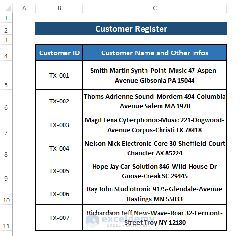
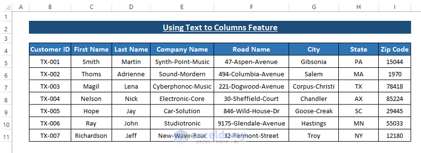
How to Split Data into Multiple Columns in Excel (5 Methods)

We’ll use the following data set to split data into multiple columns using Excel functions.

Method 1 – Using Text to Columns Feature

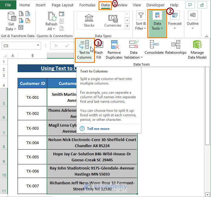
Excel provides the Text to Columns feature in the Data tab. Text to Columns features allows split data into columns separated by comma, and space that are delimiters or separating indicators.

Select the Data:
- Choose the entire column that you want to split.
- Navigate to the Data tab.
Access Text to Columns:
- Click on Data Tools.
- Select Text to Columns.

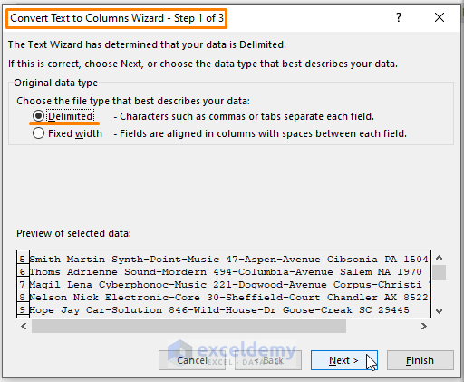
Use the Wizard:
- The Convert Text to Columns Wizard will appear.
- Choose the option that best describes your data (e.g., delimited or fixed width).
- Click Next.

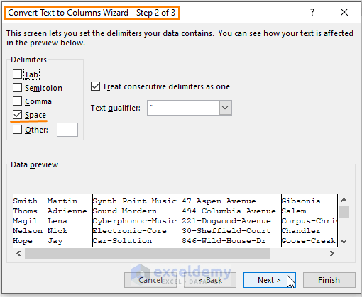
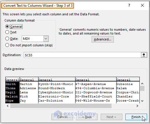
Specify Delimiters:
- If you select Delimited pick the delimiters (e.g., comma, space).
- Preview your data in the Data preview window.
- Click Next.

Set Destination:
- Choose where you want the split data to appear in your worksheet.
- Click Finish.

By following these steps, you’ll be able to split your data into separate columns as needed!

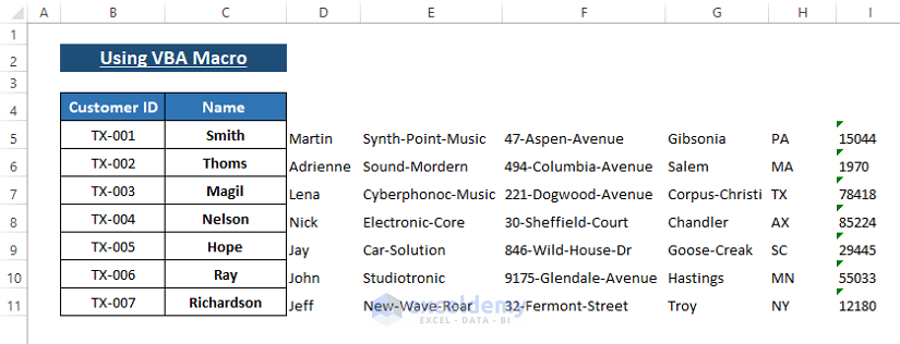
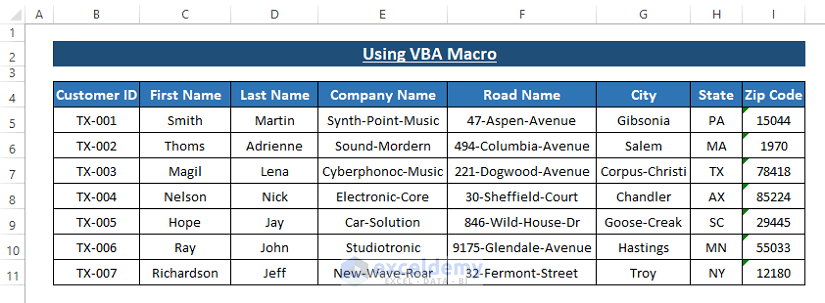
Method 2 – Using VBA Macro to Split Data into Multiple Columns

Objective:

VBA macros are effective for achieving specific outcomes.
We’ll use the VBA SPLIT function to split data from a single column into multiple columns.

Steps:

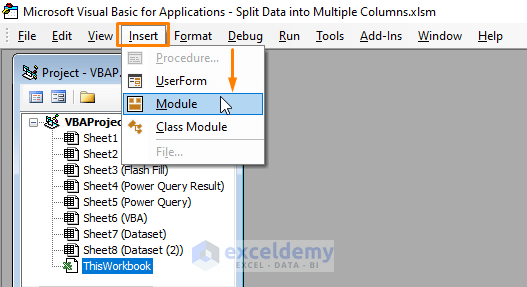
Step 1: Open the Microsoft Visual Basic Window
- Press ALT+F11 to open the Visual Basic for Applications (VBA) editor.
- Click on Insert in the toolbar and select Module.

Step 2: Paste the Macro
- In the module, paste the following VBA macro:

Sub SplitData()
For I = 5 To Cells(Rows.Count, 3).End(xlUp).Row
wrksplit = Split(Cells(I, 3).Value & " #", " ", , vbTextCompare)
Cells(I, 3).Resize(1, UBound(wrksplit)).Value = wrksplit
Next I
End Sub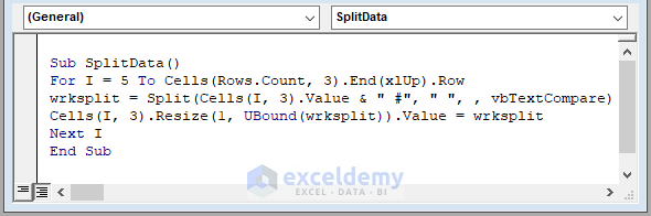

- Explanation:
  - The macro starts counting rows from row 5 up to the last used row.
  - The wrksplit variable is assigned to the VBA SPLIT function.
  - The SPLIT function uses a space as the delimiter.
  - The macro resizes the cells to match the array length using the VBA UBound function.

Step 3: Run the Macro
- Press F5 to run the macro.
- Return to your worksheet to see that the macro splits the data into multiple columns.

Customization:
- Adjust the macro outcomes according to your specific requirements.
- You can split the data into as many columns as needed by inserting spaces as separators.

Method 3 – Split Data into Multiple Columns Using Power Query

Objective:

Excel Power Query is a powerful tool for shaping data.
We’ll use Power Query Editor to split data into separate columns.

Steps:

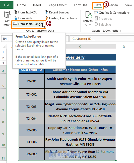
Step 1: Select the Entire Range
- Highlight the entire range of data.
- Go to the Data tab.
- Click on From Table/Range within the Get & Transform Data section.

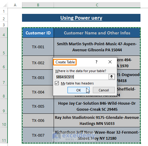
Step 2: Create Table Dialog Box
- Excel will display the Create Table dialog box.
- Depending on your data type, choose to tick or untick the My table has headers option.
- Click OK.

Step 3: Power Query Editor
- The Power Query Editor window will appear.
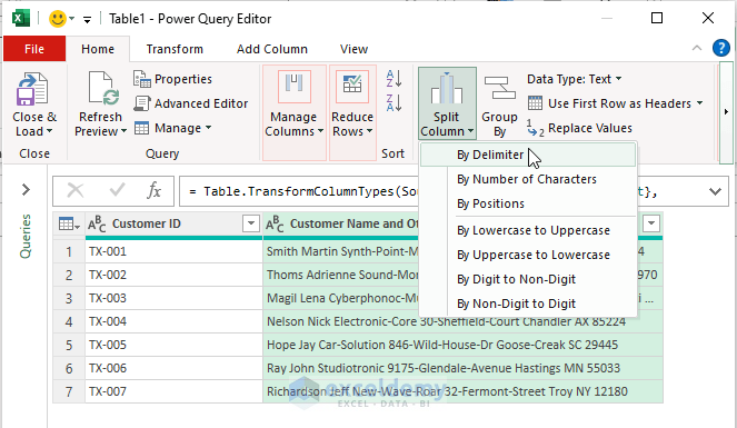
- Select the specific column containing the data you want to split.
- Go to the Home tab.
- Click on Split Column in the Transform section.
- Choose By Delimiter.

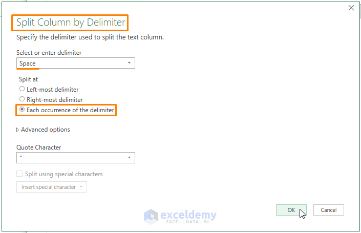
Step 4: Split Column by Delimiter
- In the dialog box:
  - Select or enter the delimiter (e.g., space).
  - Mark Each occurrence of the delimiter to split data wherever spaces exist.
  - You can choose other delimiters (e.g., comma, semicolon) as needed.
  - Click OK.

Step 5: Close & Load
- Click OK in the Split Column by Delimiter dialog box.
- The Power Query Editor will take you back to the main window.
- Click Close & Load.

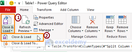
Excel will close the Power Query Editor and load the split data into your worksheet.

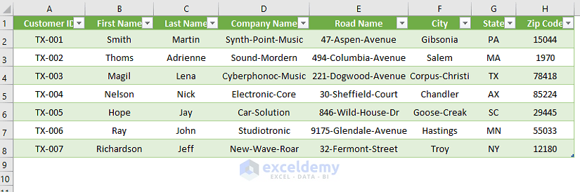
Arrange the data according to your preference.

Method 4 – Using Flash Fill to Split Data into Multiple Columns

Flash Fill is a convenient tool in Excel that allows you to quickly fill in entries based on patterns. It works by mimicking existing data and automatically filling in related information. Here’s how to use it:

First Name Separation:
- Under the First Name header, type the first entry.
- Navigate to the Home tab, then click on Editing, followed by Fill and select Flash Fill.

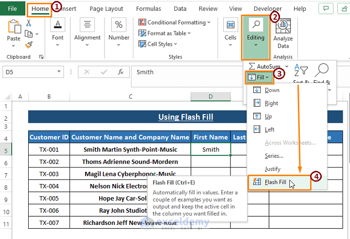
- Instantly, all other entries within the First Name column will be populated with first names. Flash Fill identifies the pattern from the first entry and fetches the corresponding words from the adjacent column

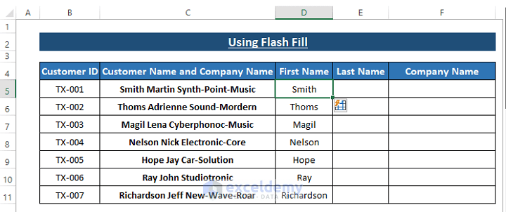
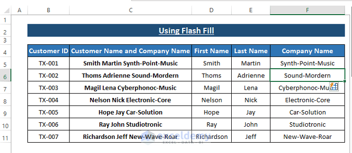
Applying to Other Columns:
- Repeat the same process for other columns, such as Last Name and Company Name.
- Note that for the Company Name column, you should provide a minimum of two entries to ensure successful Flash Fill in other cells.

Important Consideration:

Flash Fill works well for a limited variety of entries. If you have a diverse range of data, it’s advisable not to use Flash Fill, as it may incorrectly mimic the data.

Remember that Flash Fill is available in Excel 2013 and later versions1. If you’re using a Windows device, make sure to enable Flash Fill by going to “File” > “Options” > “Advanced” and checking the “Automatically Flash Fill” box.

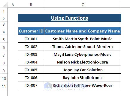
Method 5 – Splitting Data into Multiple Columns Using Functions

When working with Excel, you can extract specific portions of data from a single-entry using functions like LEFT, RIGHT, MID, SUBSTITUTE, and SEARCH. These functions allow you to manipulate text efficiently. In this method, we’ll use a simplified dataset to demonstrate how to extract information using combined functions.

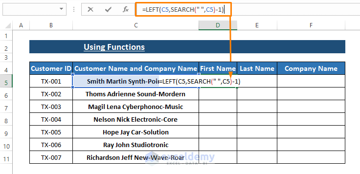
Extracting First Names:
- Begin by typing the following formula into any blank cell (e.g., D5) to extract First Names:

=LEFT(C5,SEARCH(" ",C5)-1)

- - The SEARCH function finds the position of the first space character in cell C5.
  - Subtracting 1 from this position gives us the length of the first name.
  - The LEFT function then extracts the characters up to the first space.

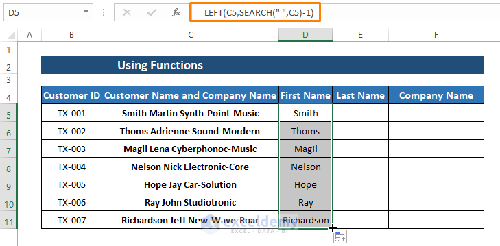
Applying the Formula:
- Press ENTER after typing the formula in cell C5.
- Drag the Fill Handle (the small square at the bottom-right corner of the cell) to apply the formula to other cells in the same column.

Inserting Last Names:
- Use the following formula to insert last names:

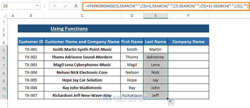
=IFERROR(MID(C5,SEARCH(" ",C5)+1,SEARCH(" ",C5,SEARCH(" ",C5)+1)-SEARCH(" ",C5)),"")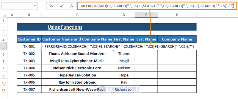

- - The SEARCH(” “,C5)+1 part determines the starting position for the MID function.
  - The expression SEARCH(” “,C5,SEARCH(” “,C5)+1)-SEARCH(” “,C5) calculates the number of characters to extract.
  - The IFERROR function prevents Excel from displaying errors when encountering a single space.

Applying the Last Name Formula:
- Press ENTER after typing the formula in the first cell.
- Drag the Fill Handle to apply the formula to other cells in the same column.

Handling Company Names:
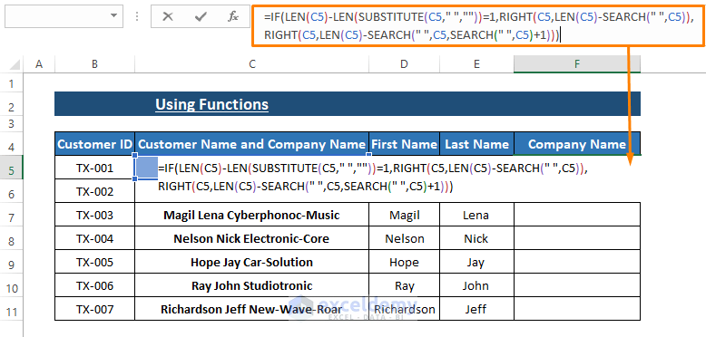
- For company names, use the following formula in respective cells:

=IF(LEN(C5)-LEN(SUBSTITUTE(C5," ",""))=1,RIGHT(C5,LEN(C5)-SEARCH(" ",C5)),RIGHT(C5,LEN(C5)-SEARCH(" ",C5,SEARCH(" ",C5)+1)))

- - The formula checks if there is only one space in the entry.
  - If true, it extracts characters using RIGHT(C5,LEN(C5)-SEARCH(” “,C5)).
  - Otherwise, it uses RIGHT(C5,LEN(C5)-SEARCH(” “,C5,SEARCH(” “,C5)+1)).

Observation from Our Data: Handling Entries with Multiple Spaces:

Based on our dataset, it’s evident that some entries contain more than one space. To address this, we use the SUBSTITUTE function to convert these entries into versions without spaces. The RIGHT function then extracts characters based on the lengths provided by the RIGHT and SEARCH functions.

Applying the Formula to the Entire Company Name Column
- Press ENTER after typing the formula in the first cell under the Company Name column.
- Drag the Fill Handle (the small square at the bottom-right corner of the cell) to apply the formula to all other cells within the same column.

Final Thoughts:

Feel free to modify any of the formulas to suit your specific dataset.
Remember that simpler methods are often more effective for splitting data into multiple columns, so avoid unnecessarily lengthy formulas.

Download Excel Workbook

You can download the practice workbook from here:

Split Data into Multiple Columns.xlsx