7 Excel Workflow Tweaks for Power Users

Image by Editor
 

Excel is an incredibly useful and powerful tool for managing and analyzing data. Excel offers numerous features and functions, but small workflow tweaks can save hours when working with complex spreadsheets.

In this tutorial, we will explore seven essential workflow tweaks for power users.

1. Use Keyboard Shortcuts to Speed Up Tasks

Keyboard shortcuts can drastically reduce the time spent navigating through Excel. Here are some essential shortcuts for power users.

• Ctrl + Shift + L: Toggle filters on or off for the current selection.
• Ctrl + Arrow Keys: Jump to the edge of data regions (up, down, left, right).
• F2: Edit the active cell.
• Alt + Enter: Create a new line within a cell.
• Alt + E, S, V: Paste special (useful for pasting only values, formats, etc.).
• Ctrl + T: Create a table from a selected range.
• Ctrl + Shift + “+”: Insert a new row or column.
• Ctrl + Shift + Arrow Keys: Select data regions.
• Ctrl + Space/Shift + Space: Select entire columns/rows.
• Alt + Down Arrow: Open dropdown lists.
• F4: Repeat the last action (great for copying formatting or operations).

By memorizing and using these shortcuts, you can streamline data manipulation and analysis significantly.

2. Leverage Excel Tables for Better Data Management

When working with large datasets, converting ranges into Excel Tables offers several advantages.

• Automatic Formatting: Tables auto-format data with alternating colors, improving readability.
• Dynamic References: Table references automatically adjust when rows are added or removed, making formulas more flexible.
• Structured Data: Tables allow for better data management with built-in filters and easy sorting.
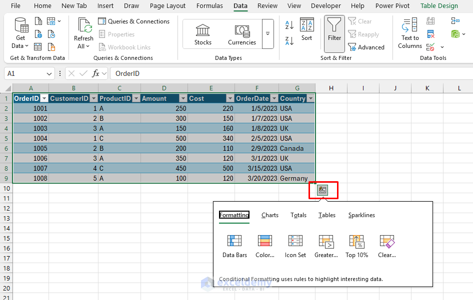
• Access Quick Analysis: Table enables quick analysis with formatting, charting, totals, sparklines, etc.

To create a table, select your data and press Ctrl + T. Afterward, you can refer to columns by their table names, making formulas easier to read and maintain.

3. Dynamic Array Formulas

Excel now supports dynamic arrays, which allow you to spill multiple results into adjacent cells with a single formula. This significantly reduces the need for manual dragging or copying formulas.

• Enter a formula like:

=SEQUENCE(5)

It generates a list of 5 sequential numbers.

• Dynamic arrays automatically fill the cells without needing to manually copy or drag the formula.

You can use the UNIQUE, FILTER, and SORT functions to instantly generate dynamic results based on specific criteria.

4. Use Power Query for Automated Data Transformation

Power Query is an essential tool for power users working with raw data.

• Import data from various sources (CSV, JSON, databases, etc.).
• Go to the Data tab >> from Get & Transform Data >> select From Table/Range.
• Clean and transform data with a few clicks.
• Combine multiple datasets from different sources.
• Refresh with one click when source data changes.

This is ideal for data that updates regularly.

5. Use Named Ranges for Easier Formula Management

Named ranges make formulas easier to read and manage. Instead of referencing a cell like B2, you can name the range something meaningful, like SalesData. This makes formulas more understandable and reduces the risk of errors when working with complex formulas.

To create a named range:

• Select the cells you want to name.
• Go to the Formulas tab >> select Name Manager.
• In the New Name box (just to the left of the formula bar), type a name.
• Click OK.

Now you can use SalesAmount in your formulas instead of cell references. This is especially helpful in large, complex spreadsheets.

Use Name Manager for Dynamic Ranges:

Instead of updating ranges manually as data grows:

• Go to the Formulas tab >> select Name Manager.
• Create a name with a formula like:

=OFFSET(Sheet1!$A$1,0,0,COUNTA(Sheet1!$A:$A),5)

• Reference this name in formulas, charts, and data validation.

6. Maximize Use of PivotTables for Data Summarization

For quickly summarizing and analyzing large datasets, PivotTables are invaluable. They allow you to dynamically analyze data, group items, and calculate totals with just a few clicks.

• Select your data range (including headers).
• Go to the Insert tab >> select PivotTable.
• In the PivotTable Field List;
• Drag and drop fields into the Rows, Columns, and Values areas to organize your data.

PivotTables allow you to create multiple views of the same data without changing the original dataset. You can also use PivotCharts for visualizing this summarized data.

7. Use VBA to Automate Repetitive Tasks

If you regularly perform repetitive tasks, writing simple VBA macros can save you significant time. VBA (Visual Basic for Applications) allows you to automate complex tasks with custom scripts.

• Go to the Developer tab >> select Visual Basic.
• Insert a new module.
• Go to the Insert tab >> select Module.
• Write a simple macro, for example:

Sub HideRows()
Rows("2:10").Hidden = True
End Sub

• Close the editor and assign the macro to a button or shortcut.

By creating a library of reusable macros, you can automate processes like formatting, data import, or even complex data analysis tasks.

Bonus Tweaks

Create Custom Views

When working with large datasets:

• Set up your window layout (frozen panes, zoom level, visible rows/columns)
• Go to View tab >> from Custom Views >> select Add.
• Name your view and save.
• Toggle between different views depending on your task.

Set Up Quick Access Toolbar

Customize your Quick Access Toolbar with your most-used commands:

• Right-click any ribbon command >> select Add to Quick Access Toolbar.
• Arrange them in order of frequency of use.
• Consider adding:
  • Camera Tool.
  • Format Painter.
  • Sort, Filter.
  • Text to Columns.

Final Thoughts

By implementing these seven workflow tweaks, you can elevate your Excel productivity and efficiency. Power users not only focus on performing tasks faster but also on improving the accuracy and consistency of their work. You can start by automating simple tasks with macros or exploring Power Query to streamline your data transformation processes.